自编码器AutoEncoder
文章目录
- 一. 什么是自编码器
- 二. 有什么作用
- 1) 图像去噪
- 2) 可视化降维
- 三. 如何实现
- 1) 全连接层实现
- 2) 测试: 对有噪声图像的自编码
- 3) 卷积层实现
- 四. 一些小细节
一. 什么是自编码器
自动编码器 autoencoder, 简单表现编码器为将一组数据进行压缩编码(降维), 解码器将这组数据恢复成高维的数据. 这种编码和解码的过程不是无损的, 因此最终的输出和输入是有一些差异的, 且非常依赖于训练的数据集.
如图所示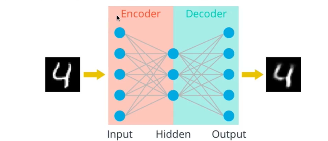
如上面这张图所示, 对于一个简单的三层线性神经网络组成的自编码器, 我们在进行神经网络的搭建过程中, 将(input, hidden) 这个过程叫做编码器, 将(hidden, output) 这个过程叫做解码器. 对于mnist数据集而言, 它的维度变化是 784 -> x -> 784, 其中, x < 784, 是编码的维度.
二. 有什么作用
1) 图像去噪
看上去很强啊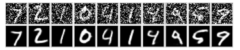
2) 可视化降维
三. 如何实现
训练神经网络需要定义损失函数, 那么这个自编码器的损失衡量值是什么?
衡量损失的值是由网络的输出结果和输入决定的. 也就是说, 是由这两个784维数据的差别决定的.
1) 全连接层实现
首先定义一个神经网络
class Autoencoder(nn.Module):def __init__(self, encoding_dim):super(Autoencoder, self).__init__()## encoder ##self.encoder = nn.Linear(784, encoding_dim)## decoder ##self.decoder = nn.Linear(encoding_dim, 784)def forward(self, x):# define feedforward behavior# and scale the *output* layer with a sigmoid activation function# print(x.shape)x = x.view(-1, 784)x = F.relu(self.encoder(x))x = torch.sigmoid(self.decoder(x))return x# initialize the NNencoding_dim = 128model = Autoencoder(encoding_dim)
定义损失函数和优化器
# specify loss functioncriterion = nn.MSELoss()# specify loss functionoptimizer = torch.optim.Adam(model.parameters(), lr=0.001)
训练过程, 一共20个epochs, 话说pytorch还真慢, 这么简单的网络都要训练好一会
# number of epochs to train the modeln_epochs = 20for epoch in range(1, n_epochs+1):# monitor training losstrain_loss = 0.0#################### train the model ####################for data in train_loader:# _ stands in for labels, hereimages, _ = data# flatten imagesimages = images.view(images.size(0), -1)# clear the gradients of all optimized variablesoptimizer.zero_grad()# forward pass: compute predicted outputs by passing inputs to the model# print(images.shape)outputs = model(images)# calculate the lossloss = criterion(outputs, images)# backward pass: compute gradient of the loss with respect to model parametersloss.backward()# perform a single optimization step (parameter update)optimizer.step()# update running training losstrain_loss += loss.item()*images.size(0)# print avg training statisticstrain_loss = train_loss/len(train_loader)print('Epoch: {} \tTraining Loss: {:.6f}'.format(epoch,train_loss))
训练过程的损失变化
Epoch: 1 Training Loss: 0.342308Epoch: 2 Training Loss: 0.081272Epoch: 3 Training Loss: 0.058724Epoch: 4 Training Loss: 0.051274Epoch: 5 Training Loss: 0.047382Epoch: 6 Training Loss: 0.044760Epoch: 7 Training Loss: 0.043184Epoch: 8 Training Loss: 0.042066Epoch: 9 Training Loss: 0.041246Epoch: 10 Training Loss: 0.040589Epoch: 11 Training Loss: 0.040059Epoch: 12 Training Loss: 0.039646Epoch: 13 Training Loss: 0.039272Epoch: 14 Training Loss: 0.038980Epoch: 15 Training Loss: 0.038733Epoch: 16 Training Loss: 0.038524Epoch: 17 Training Loss: 0.038328Epoch: 18 Training Loss: 0.038162Epoch: 19 Training Loss: 0.038012Epoch: 20 Training Loss: 0.037874
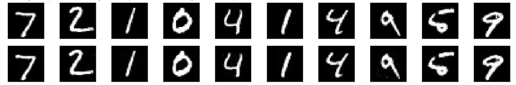
那么效果如何呢? 上面一排是输入图像, 下面一排是输出图像. 经过自编码器之后, 还原度还是很高的.
2) 测试: 对有噪声图像的自编码
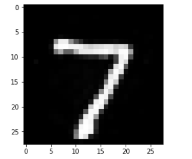
首先查看一张图片
a_img = np.squeeze(images[0])print(a_img.shape)print(np.max(a_img))print(np.min(a_img))plt.imshow(a_img, cmap='gray')
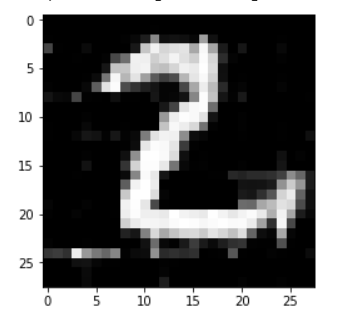
然后向其中加入噪声
a_img_x = a_img + 0.08 * np.random.normal(loc=0.0, scale=1.0, size=a_img.shape)plt.imshow(a_img_x, cmap='gray')
这是加入噪声之后的图片, 可以看出差别还是很大的. 那么我们的编码器能还原出如何的效果呢?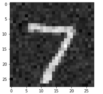
a_img_output = model(torch.Tensor(a_img_x).view(1, -1))print(a_img_output.shape)output_img = a_img_output.view(28, 28)output_img = output_img.detach().numpy()plt.imshow(output_img, cmap='gray')
这是还原后的, 说实话看到这个图片我心里也是很惊讶的. 就在于加入那么多噪声之后, 居然还可以还原的如此清晰. 当然这是对于MNIST数据集而言, 这个数据集比较简单.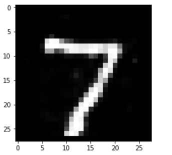
3) 卷积层实现
不同之处在于定义自编码器的神经网络结构
如图所示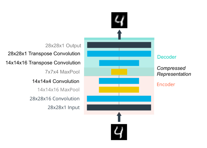
可以看到在decoder中经过了两个反卷积层, 但是由于水平有限, 这个反卷积层看着好奇怪, 不知道是怎么反卷积的.
pytorch实现
import torch.nn as nnimport torch.nn.functional as F# define the NN architectureclass ConvAutoencoder(nn.Module):def __init__(self):super(ConvAutoencoder, self).__init__()## encoder layers ##self.conv1 = nn.Conv2d(1, 16, 3, padding=1)self.conv2 = nn.Conv2d(16, 4, 3, padding=1)self.pool = nn.MaxPool2d(2, 2)## decoder layers #### a kernel of 2 and a stride of 2 will increase the spatial dims by 2self.t_conv1 = nn.ConvTranspose2d(4, 16, 2, stride=2)self.t_conv2 = nn.ConvTranspose2d(16, 1, 2, stride=2)def forward(self, x):## encode #### decode #### apply ReLu to all hidden layers *except for the output layer## apply a sigmoid to the output layerx = F.relu(self.conv1(x))x = self.pool(x)x = F.relu(self.conv2(x))x = self.pool(x)x = F.relu(self.t_conv1(x))x = torch.sigmoid(self.t_conv2(x))return x# initialize the NNmodel = ConvAutoencoder()print(model)
训练起来比全连接层的网络还要慢很多, 而损失值的降低也慢很多, 不像之前从epoch 1 到 epoch 2 直接就断崖式下跌了. 下面是损失值的变化过程, 只训练了 15个epoch. 从损失之上看这个效果好像差很多?
Epoch: 1 Training Loss: 0.448799Epoch: 2 Training Loss: 0.266815Epoch: 3 Training Loss: 0.251290Epoch: 4 Training Loss: 0.240823Epoch: 5 Training Loss: 0.231836Epoch: 6 Training Loss: 0.220550Epoch: 7 Training Loss: 0.210341Epoch: 8 Training Loss: 0.202768Epoch: 9 Training Loss: 0.197010Epoch: 10 Training Loss: 0.193259Epoch: 11 Training Loss: 0.190589Epoch: 12 Training Loss: 0.188406Epoch: 13 Training Loss: 0.186529Epoch: 14 Training Loss: 0.184983Epoch: 15 Training Loss: 0.183579
观察下图的数字9的话, 可以看到损失了不少.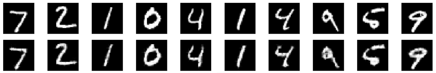
再看看噪声图片的处理能力如何
原图: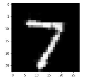
加入噪声: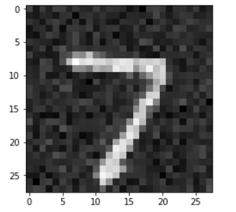
经过自编码器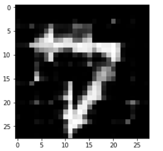
呃, 效果似乎有点不是很对, 可能是训练的epoch太少了, 毕竟我们可以前面看到训练15个epoch的损失值还是达到了0.18, 而在全连接层的简单自编码器上第二个epoch的损失值就达到了0.08
另一张图片
噪声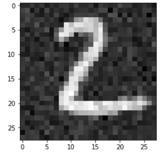
四. 一些小细节
- numpy 的 squeeze 函数
参考博客
作用:从数组的形状中删除单维度条目,即把shape中为1的维度去掉 给MNIST图片加入噪声的方法
test_img_x = test_img + 0.08 * np.random.normal(loc=0.0, scale=1.0, size=test_img.shape)
就是加入一些随机值, 在原图的基础上进行小幅度修改.


")
MySQL Protocol和Read调用栈")


还没有评论,来说两句吧...