pytorch:多项式回归
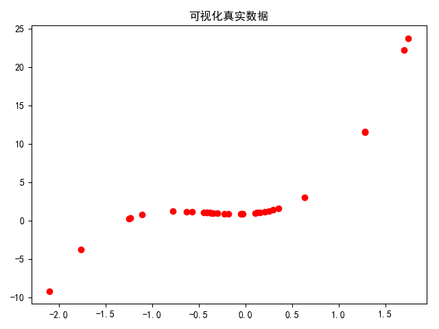
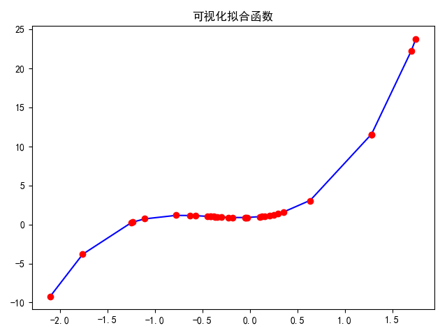
import numpy as npimport torchfrom torch.autograd import Variablefrom torch import nn, optimimport matplotlib.pyplot as plt# 设置字体为中文plt.rcParams['font.sans-serif'] = ['SimHei']plt.rcParams['axes.unicode_minus'] = False# 构造成次方矩阵def make_fertures(x):x = x.unsqueeze(1)return torch.cat([x ** i for i in range(1, 4)], 1)# y = 0.9+0.5*x+3*x*x+2.4x*x*xW_target = torch.FloatTensor([0.5, 3, 2.4]).unsqueeze(1)b_target = torch.FloatTensor([0.9])# 计算x*w+bdef f(x):return x.mm(W_target) + b_target.item()def get_batch(batch_size=32):random = torch.randn(batch_size)random = np.sort(random)random = torch.Tensor(random)x = make_fertures(random)y = f(x)if (torch.cuda.is_available()):return Variable(x).cuda(), Variable(y).cuda()else:return Variable(x), Variable(y)# 多项式模型class poly_model(nn.Module):def __init__(self):super(poly_model, self).__init__()self.poly = nn.Linear(3, 1) # 输入时3维,输出是1维def forward(self, x):out = self.poly(x)return outif torch.cuda.is_available():model = poly_model().cuda()else:model = poly_model()# 均方误差,随机梯度下降criterion = nn.MSELoss()optimizer = optim.SGD(model.parameters(), lr=1e-3)epoch = 0 # 统计训练次数ctn = []lo = []while True:batch_x, batch_y = get_batch()output = model(batch_x)loss = criterion(output, batch_y)print_loss = loss.item()optimizer.zero_grad()loss.backward()optimizer.step()ctn.append(epoch)lo.append(print_loss)epoch += 1if (print_loss < 1e-3):breakprint("Loss: {:.6f} after {} batches".format(loss.item(), epoch))print("==> Learned function: y = {:.2f} + {:.2f}*x + {:.2f}*x^2 + {:.2f}*x^3".format(model.poly.bias[0], model.poly.weight[0][0],model.poly.weight[0][1],model.poly.weight[0][2]))print("==> Actual function: y = {:.2f} + {:.2f}*x + {:.2f}*x^2 + {:.2f}*x^3".format(b_target[0], W_target[0][0],W_target[1][0], W_target[2][0]))# 1.可视化真实数据predict = model(batch_x)x = batch_x.numpy()[:, 0] # x~1 x~2 x~3plt.plot(x, batch_y.numpy(), 'ro')plt.title(label='可视化真实数据')plt.show()# 2.可视化拟合函数predict = predict.data.numpy()plt.plot(x, predict, 'b')plt.plot(x, batch_y.numpy(), 'ro')plt.title(label='可视化拟合函数')plt.show()# 3.可视化训练次数和损失plt.plot(ctn,lo)plt.xlabel('训练次数')plt.ylabel('损失值')plt.title(label='训练次数与损失关系')plt.show()
实验结果:
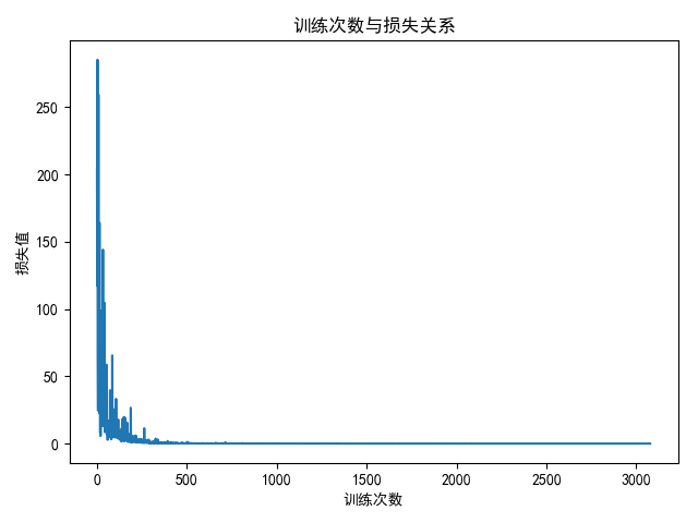
注意:批量产生数据后,进行一个排序,否则可视化时,不是按照x轴从小到大绘制,出现很多折线。对应代码:
random = np.sort(random)random = torch.Tensor(random)


.nw执行过程及如何获取.nw真实路径")


还没有评论,来说两句吧...