最小二乘法的多元线性回归-蒲公英云

最小二乘法的多元线性回归

方法介绍

“最小二乘法”一句话解释：一种数学优化方法，通过最小化误差的平方和来寻找合适的数据拟合函数。
线性模型的最小二乘可以有很多方法来实现，比如直接使用矩阵运算求解析解，sklearn包（参考：用scikit-learn和pandas学习线性回归、用scikit-learn求解多元线性回归问题），或scipy里的leastsq function（参考：How to use leastsq function from scipy.optimize ）。

具体问题代码实现

数据

这里写图片描述

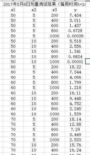
代码

本文使用scipy的leastsq函数实现，代码如下。

from scipy.optimize import leastsq
import numpy as np
def main():
    # data provided
    x = np.array([[1, 50, 5, 200], [1, 50, 5, 400], [1, 50, 5, 600], [1, 50, 5, 800], [1, 50, 5, 1000],
                 [1, 50, 10, 200], [1, 50, 10, 400], [1, 50, 10, 600], [1, 50, 10, 800], [1, 50, 10, 1000],
                 [1, 60, 5, 200], [1, 60, 5, 400], [1, 60, 5, 600], [1, 60, 5, 800], [1, 60, 5, 1000],
                 [1, 60, 10, 200], [1, 60, 10, 400], [1, 60, 10, 600], [1, 60, 10, 800], [1, 60, 10, 1000],
                 [1, 70, 5, 200], [1, 70, 5, 400], [1, 70, 5, 600], [1, 70, 5, 800], [1, 70, 5, 1000],
                 [1, 70, 10, 200], [1, 70, 10, 400]])
    y = np.array([7.434, 3.011, 1.437, 0.6728, 0.00036,
               5.518, 2.556, 1.341, 0.6824, 0.0001,
               18.22, 7.344, 4.066, 1.799, 1.218,
               16.11, 9.448, 4.752, 2.245, 1.539,
               18.14, 12.88, 7.29, 3.449, 2.533,
               15.76, 16.24])
    # here, create lambda functions for Line fit
    # tpl is a tuple that contains the parameters of the fit
    funcLine=lambda tpl,x: np.dot(x, tpl)
    # func is going to be a placeholder for funcLine,funcQuad or whatever
    # function we would like to fit
    func = funcLine
    # ErrorFunc is the diference between the func and the y "experimental" data
    ErrorFunc = lambda tpl, x, y: func(tpl, x)-y
    #tplInitial contains the "first guess" of the parameters
    tplInitial=[1.0, 1.0, 1.0, 1.0]
    # leastsq finds the set of parameters in the tuple tpl that minimizes
    # ErrorFunc=yfit-yExperimental
    tplFinal, success = leastsq(ErrorFunc, tplInitial, args=(x, y))
    print('linear fit', tplFinal)
    print(funcLine(tplFinal, x))
if __name__ == "__main__":
   main()

实验结果及分析

实验结果

# tplFinal值
[-8.43371266  0.3787503   0.11744081 -0.01485372]
# y预测值
[  8.12026253   5.1495184    2.17877428  -0.79196984  -3.76271396
   8.70746659   5.73672247   2.76597835  -0.20476577  -3.17550989
  11.90776557   8.93702145   5.96627733   2.99553321   0.02478909
  12.49496964   9.52422552   6.5534814    3.58273728   0.61199315
  15.69526862  12.7245245    9.75378038   6.78303626   3.81229214
  16.28247269  13.31172857]

分析总结

a) 从结果可以看出使用线性模型拟合的效果并不是特别好，可进一步尝试使用二次曲线等较复杂模型。
b) 拟合直线应首先自己观察一下给定数据x、y之间是否有什么关系。比如上述所给数据明显是一个基于控制变量的对照组实验，先观察一下其自变量（特征）与因变量（目标）之间的关系，你会明显发现自变量x3(200, 400, 600...)与y值成负相关。这样至少心里有个底儿。
c) 感觉使用scipy的leastsq函数来做并不是那么方便，下次可尝试使用sklearn包。