Best packages for data manipulation in R
There are 2 packages that make data manipulation in R fun. These are dplyr and data.table. Both packages have their strengths. While dplyr is more elegant and resembles natural language,data.table is succinct and we can do a lot with data.table in just a single line. Further, data.table is, in some cases, faster (see benchmark here) and it may be a go-to package when performance and memory are constraints. You can read comparison of dplyr and data.table from Stack Overflow andQuora.
You can get reference manual and vignettes for data.table hereand for dplyr here. You can read other tutorial about dplyrpublished at DataScience+
Background
I am a long time dplyr and data.table user for my data manipulation tasks. For someone who knows one of these packages, I thought it could help to show codes that perform the same tasks in both packages to help them quickly study the other. If you know either package and have interest to study the other, this post is for you.
dplyr
dplyr has 5 verbs which make up the majority of the data manipulation tasks we perform. Select: used to select one or more columns; Filter: used to select some rows based on specific criteria; Arrange: used to sort data based on one or more columns in ascending or descending order; Mutate: used to add new columns to our data; Summarise: used to create chunks from our data.
data.table
data.table has a very succinct general format: DT[i, j, by], which is interpreted as: Take DT, subset rows using i, then calculate jgrouped by by.
Data manipulation
First we will install some packages for our project.
library(dplyr)library(data.table)library(lubridate)library(jsonlite)library(tidyr)library(ggplot2)library(compare)
The data we will use here is from DATA.GOV. It is Medicare Hospital Spending by Claim and it can be downloaded from here. Let’s download the data in JSON format using the fromJSON function from the jsonlite package. Since JSON is a very common data format used for asynchronous browser/server communication, it is good if you understand the lines of code below used to get the data. You can get an introductory tutorial on how to use the jsonlite package to work with JSON data here and here. However, if you want to focus only on the data.table and dplyr commands, you can safely just run the codes in the two cells below and ignore the details.
spending=fromJSON("https://data.medicare.gov/api/views/nrth-mfg3/rows.json?accessType=DOWNLOAD")names(spending)"meta" "data"meta=spending$metahospital_spending=data.frame(spending$data)colnames(hospital_spending)=make.names(meta$view$columns$name)hospital_spending=select(hospital_spending,-c(sid:meta))glimpse(hospital_spending)Observations: 70598Variables:$ Hospital.Name (fctr) SOUTHEAST ALABAMA MEDICAL CENT...$ Provider.Number. (fctr) 010001, 010001, 010001, 010001...$ State (fctr) AL, AL, AL, AL, AL, AL, AL, AL...$ Period (fctr) 1 to 3 days Prior to Index Hos...$ Claim.Type (fctr) Home Health Agency, Hospice, I...$ Avg.Spending.Per.Episode..Hospital. (fctr) 12, 1, 6, 160, 1, 6, 462, 0, 0...$ Avg.Spending.Per.Episode..State. (fctr) 14, 1, 6, 85, 2, 9, 492, 0, 0,...$ Avg.Spending.Per.Episode..Nation. (fctr) 13, 1, 5, 117, 2, 9, 532, 0, 0...$ Percent.of.Spending..Hospital. (fctr) 0.06, 0.01, 0.03, 0.84, 0.01, ...$ Percent.of.Spending..State. (fctr) 0.07, 0.01, 0.03, 0.46, 0.01, ...$ Percent.of.Spending..Nation. (fctr) 0.07, 0.00, 0.03, 0.58, 0.01, ...$ Measure.Start.Date (fctr) 2014-01-01T00:00:00, 2014-01-0...$ Measure.End.Date (fctr) 2014-12-31T00:00:00, 2014-12-3...
As shown above, all columns are imported as factors and let’s change the columns that contain numeric values to numeric.
cols = 6:11; # These are the columns to be changed to numeric.hospital_spending[,cols] <- lapply(hospital_spending[,cols], as.numeric)
The last two columns are measure start date and measure end date. So, let’s use the lubridate package to correct the classes of these columns.
cols = 12:13; # These are the columns to be changed to dates.hospital_spending[,cols] <- lapply(hospital_spending[,cols], ymd_hms)
Now, let’s check if the columns have the classes we want.
sapply(hospital_spending, class)$Hospital.Name"factor"$Provider.Number."factor"$State"factor"$Period"factor"$Claim.Type"factor"$Avg.Spending.Per.Episode..Hospital."numeric"$Avg.Spending.Per.Episode..State."numeric"$Avg.Spending.Per.Episode..Nation."numeric"$Percent.of.Spending..Hospital."numeric"$Percent.of.Spending..State."numeric"$Percent.of.Spending..Nation."numeric"$Measure.Start.Date"POSIXct" "POSIXt"$Measure.End.Date"POSIXct" "POSIXt"
Create data table
We can create a data.table using the data.table() function.
hospital_spending_DT = data.table(hospital_spending)class(hospital_spending_DT)"data.table" "data.frame"
Select certain columns of data
To select columns, we use the verb select in dplyr. Indata.table, on the other hand, we can specify the column names.
Selecting one variable
Let’s selet the “Hospital Name” variable
from_dplyr = select(hospital_spending, Hospital.Name)from_data_table = hospital_spending_DT[,.(Hospital.Name)]
Now, let’s compare if the results from dplyr and data.table are the same.
compare(from_dplyr,from_data_table, allowAll=TRUE)TRUEdropped attributes
Removing one variable
from_dplyr = select(hospital_spending, -Hospital.Name)from_data_table = hospital_spending_DT[,!c("Hospital.Name"),with=FALSE]compare(from_dplyr,from_data_table, allowAll=TRUE)TRUEdropped attributes
we can also use := function which modifies the input data.tableby reference.
We will use the copy()function, which deep copies the input object and therefore any subsequent update by reference operations performed on the copied object will not affect the original object.
DT=copy(hospital_spending_DT)DT=DT[,Hospital.Name:=NULL]"Hospital.Name"%in%names(DT)FALSE
We can also remove many variables at once similarly:
DT=copy(hospital_spending_DT)DT=DT[,c("Hospital.Name","State","Measure.Start.Date","Measure.End.Date"):=NULL]c("Hospital.Name","State","Measure.Start.Date","Measure.End.Date")%in%names(DT)FALSE FALSE FALSE FALSE
Selecting multiple variables
Let’s select the variables:
Hospital.Name,State,Measure.Start.Date,and Measure.End.Date.
from_dplyr = select(hospital_spending, Hospital.Name,State,Measure.Start.Date,Measure.End.Date)from_data_table = hospital_spending_DT[,.(Hospital.Name,State,Measure.Start.Date,Measure.End.Date)]compare(from_dplyr,from_data_table, allowAll=TRUE)TRUEdropped attributes
Dropping multiple variables
Now, let’s remove the variables Hospital.Name,State,Measure.Start.Date,and Measure.End.Date from the original data frame hospital_spending and the data.table hospital_spending_DT.
from_dplyr = select(hospital_spending, -c(Hospital.Name,State,Measure.Start.Date,Measure.End.Date))from_data_table = hospital_spending_DT[,!c("Hospital.Name","State","Measure.Start.Date","Measure.End.Date"),with=FALSE]compare(from_dplyr,from_data_table, allowAll=TRUE)TRUEdropped attributes
dplyr has functions contains(), starts_with() and,ends_with() which we can use with the verb select. Indata.table, we can use regular expressions. Let’s select columns that contain the word Date to demonstrate by example.
from_dplyr = select(hospital_spending,contains("Date"))from_data_table = subset(hospital_spending_DT,select=grep("Date",names(hospital_spending_DT)))compare(from_dplyr,from_data_table, allowAll=TRUE)TRUEdropped attributesnames(from_dplyr)"Measure.Start.Date" "Measure.End.Date"
Rename columns
setnames(hospital_spending_DT,c("Hospital.Name", "Measure.Start.Date","Measure.End.Date"), c("Hospital","Start_Date","End_Date"))names(hospital_spending_DT)"Hospital" "Provider.Number." "State" "Period" "Claim.Type" "Avg.Spending.Per.Episode..Hospital." "Avg.Spending.Per.Episode..State." "Avg.Spending.Per.Episode..Nation." "Percent.of.Spending..Hospital." "Percent.of.Spending..State." "Percent.of.Spending..Nation." "Start_Date" "End_Date"hospital_spending = rename(hospital_spending,Hospital= Hospital.Name, Start_Date=Measure.Start.Date,End_Date=Measure.End.Date)compare(hospital_spending,hospital_spending_DT, allowAll=TRUE)TRUEdropped attributes
Filtering data to select certain rows
To filter data to select specific rows, we use the verb filter fromdplyr with logical statements that could include regular expressions. In data.table, we need the logical statements only.
Filter based on one variable
from_dplyr = filter(hospital_spending,State=='CA') # selecting rows for Californiafrom_data_table = hospital_spending_DT[State=='CA']compare(from_dplyr,from_data_table, allowAll=TRUE)TRUEdropped attributes
Filter based on multiple variables
from_dplyr = filter(hospital_spending,State=='CA' & Claim.Type!="Hospice")from_data_table = hospital_spending_DT[State=='CA' & Claim.Type!="Hospice"]compare(from_dplyr,from_data_table, allowAll=TRUE)TRUEdropped attributesfrom_dplyr = filter(hospital_spending,State %in% c('CA','MA',"TX"))from_data_table = hospital_spending_DT[State %in% c('CA','MA',"TX")]unique(from_dplyr$State)CA MA TXcompare(from_dplyr,from_data_table, allowAll=TRUE)TRUEdropped attributes
Order data
We use the verb arrange in dplyr to order the rows of data. We can order the rows by one or more variables. If we want descending, we have to use desc() as shown in the examples.The examples are self-explanatory on how to sort in ascending and descending order. Let’s sort using one variable.
Ascending
from_dplyr = arrange(hospital_spending, State)from_data_table = setorder(hospital_spending_DT, State)compare(from_dplyr,from_data_table, allowAll=TRUE)TRUEdropped attributes
Descending
from_dplyr = arrange(hospital_spending, desc(State))from_data_table = setorder(hospital_spending_DT, -State)compare(from_dplyr,from_data_table, allowAll=TRUE)TRUEdropped attributes
Sorting with multiple variables
Let’s sort with State in ascending order and End_Date in descending order.
from_dplyr = arrange(hospital_spending, State,desc(End_Date))from_data_table = setorder(hospital_spending_DT, State,-End_Date)compare(from_dplyr,from_data_table, allowAll=TRUE)TRUEdropped attributes
Adding/updating column(s)
In dplyr we use the function mutate() to add columns. Indata.table, we can Add/update a column by reference using :=in one line.
from_dplyr = mutate(hospital_spending, diff=Avg.Spending.Per.Episode..State. - Avg.Spending.Per.Episode..Nation.)from_data_table = copy(hospital_spending_DT)from_data_table = from_data_table[,diff := Avg.Spending.Per.Episode..State. - Avg.Spending.Per.Episode..Nation.]compare(from_dplyr,from_data_table, allowAll=TRUE)TRUEsortedrenamed rowsdropped row namesdropped attributesfrom_dplyr = mutate(hospital_spending, diff1=Avg.Spending.Per.Episode..State. - Avg.Spending.Per.Episode..Nation.,diff2=End_Date-Start_Date)from_data_table = copy(hospital_spending_DT)from_data_table = from_data_table[,c("diff1","diff2") := list(Avg.Spending.Per.Episode..State. - Avg.Spending.Per.Episode..Nation.,diff2=End_Date-Start_Date)]compare(from_dplyr,from_data_table, allowAll=TRUE)TRUEdropped attributes
Summarizing columns
We can use the summarize() function fromdplyrto create summary statistics.
summarize(hospital_spending,mean=mean(Avg.Spending.Per.Episode..Nation.))mean 8.772727hospital_spending_DT[,.(mean=mean(Avg.Spending.Per.Episode..Nation.))]mean 8.772727summarize(hospital_spending,mean=mean(Avg.Spending.Per.Episode..Nation.),maximum=max(Avg.Spending.Per.Episode..Nation.),minimum=min(Avg.Spending.Per.Episode..Nation.),median=median(Avg.Spending.Per.Episode..Nation.))mean maximum minimum median8.77 19 1 8.5hospital_spending_DT[,.(mean=mean(Avg.Spending.Per.Episode..Nation.),maximum=max(Avg.Spending.Per.Episode..Nation.),minimum=min(Avg.Spending.Per.Episode..Nation.),median=median(Avg.Spending.Per.Episode..Nation.))]mean maximum minimum median8.77 19 1 8.5
We can calculate our summary statistics for some chunks separately. We use the function group_by() in dplyr and indata.table, we simply provide by.
head(hospital_spending_DT[,.(mean=mean(Avg.Spending.Per.Episode..Hospital.)),by=.(Hospital)])
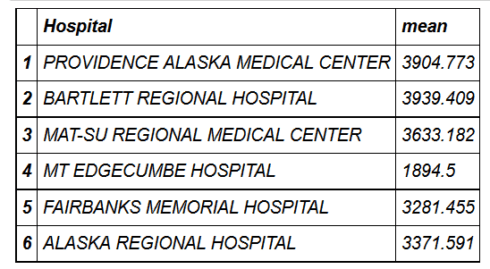
mygroup= group_by(hospital_spending,Hospital)from_dplyr = summarize(mygroup,mean=mean(Avg.Spending.Per.Episode..Hospital.))from_data_table=hospital_spending_DT[,.(mean=mean(Avg.Spending.Per.Episode..Hospital.)), by=.(Hospital)]compare(from_dplyr,from_data_table, allowAll=TRUE)TRUEsortedrenamed rowsdropped row namesdropped attributes
We can also provide more than one grouping condition.
head(hospital_spending_DT[,.(mean=mean(Avg.Spending.Per.Episode..Hospital.)),by=.(Hospital,State)])
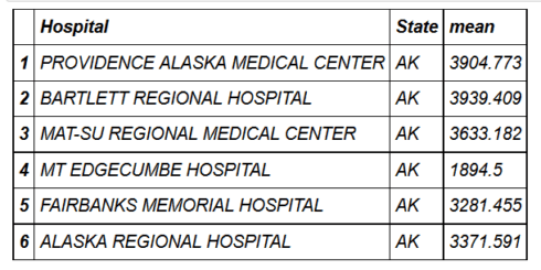
mygroup= group_by(hospital_spending,Hospital,State)from_dplyr = summarize(mygroup,mean=mean(Avg.Spending.Per.Episode..Hospital.))from_data_table=hospital_spending_DT[,.(mean=mean(Avg.Spending.Per.Episode..Hospital.)), by=.(Hospital,State)]compare(from_dplyr,from_data_table, allowAll=TRUE)TRUEsortedrenamed rowsdropped row namesdropped attributes
Chaining
With both dplyr and data.table, we can chain functions in succession. In dplyr, we use pipes from the magrittr package with %>% which is really cool. %>%takes the output from one function and feeds it to the first argument of the next function. Indata.table, we can use %>% or [ for chaining.
from_dplyr=hospital_spending%>%group_by(Hospital,State)%>%summarize(mean=mean(Avg.Spending.Per.Episode..Hospital.))from_data_table=hospital_spending_DT[,.(mean=mean(Avg.Spending.Per.Episode..Hospital.)), by=.(Hospital,State)]compare(from_dplyr,from_data_table, allowAll=TRUE)TRUEsortedrenamed rowsdropped row namesdropped attributeshospital_spending%>%group_by(State)%>%summarize(mean=mean(Avg.Spending.Per.Episode..Hospital.))%>%arrange(desc(mean))%>%head(10)%>%mutate(State = factor(State,levels = State[order(mean,decreasing =TRUE)]))%>%ggplot(aes(x=State,y=mean))+geom_bar(stat='identity',color='darkred',fill='skyblue')+xlab("")+ggtitle('Average Spending Per Episode by State')+ylab('Average')+ coord_cartesian(ylim = c(3800, 4000))
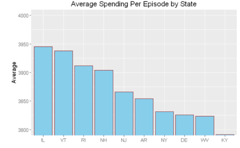
hospital_spending_DT[,.(mean=mean(Avg.Spending.Per.Episode..Hospital.)),by=.(State)][order(-mean)][1:10]%>%mutate(State = factor(State,levels = State[order(mean,decreasing =TRUE)]))%>%ggplot(aes(x=State,y=mean))+geom_bar(stat='identity',color='darkred',fill='skyblue')+xlab("")+ggtitle('Average Spending Per Episode by State')+ylab('Average')+ coord_cartesian(ylim = c(3800, 4000))
Summary
In this blog post, we saw how we can perform the same tasks usingdata.table and dplyr packages. Both packages have their strengths. While dplyr is more elegant and resembles natural language, data.table is succinct and we can do a lot withdata.tablein just a single line. Further, data.table is, in some cases, faster and it may be a go-to package when performance and memory are the constraints.
You can get the code for this blog post at my GitHub account.
This is enough for this post. If you have any questions or feedback, feel free to leave a comment.
Related Post
- Identify, describe, plot, and remove the outliers from the dataset
- Learn R By Intensive Practice – Part 2
- Working with databases in R
- Data manipulation with tidyr
- Bringing the powers of SQL into R


类似于ArcScan提取道路中心线")


还没有评论,来说两句吧...