这里采用沪深300指数数据，时间跨度为2010-10-10至今，选择每天最高价格。假设当天最高价依赖当天的前n（如30）天的沪深300的最高价。用LSTM模型来捕捉最高价的时序信息，通过训练模型，使之学会用前n天的最高价，判断当天的最高价（作为训练的标签值）。

导入数据

这里使用tushare来下载沪深300指数数据。可以用pip 安装tushare。

import tushare as ts  #导入
cons = ts.get_apis()   #建立连接
#获取沪深指数(000300)的信息，包括交易日期（datetime）、开盘价(open)、收盘价(close)，
#最高价(high)、最低价(low)、成交量(vol)、成交金额(amount)、涨跌幅(p_change)
df = ts.bar('000300', conn=cons, asset='INDEX', start_date='2010-01-01', end_date='')
#删除有null值的行
df = df.dropna()
#把df保存到当前目录下的sh300.csv文件中，以便后续使用
df.to_csv('sh300.csv')
本接口即将停止更新，请尽快使用Pro版接口：https://waditu.com/document/2

数据概览

（1）查看下载数据的字段、统计信息等。

#查看df涉及的列名
print(df.columns)
# Index(['code', 'open', 'close', 'high', 'low', 'vol', 'amount', 'p_change'], #dtype='object')
#查看df的统计信息
df.describe()
Index(['code', 'open', 'close', 'high', 'low', 'vol', 'amount', 'p_change'], dtype='object')

	open	close	high	low	vol	amount	p_change
count	2795.000000	2795.000000	2795.000000	2795.000000	2.795000e+03	2.795000e+03	2795.000000
mean	3342.024819	3344.784845	3370.611827	3314.019947	1.146134e+06	1.499518e+11	0.023324
std	809.944990	810.070118	816.521375	800.923783	8.775841e+05	1.306605e+11	1.448982
min	2079.870000	2086.970000	2118.790000	2023.170000	2.190120e+05	2.120044e+10	-8.750000
25%	2618.540000	2620.265000	2645.770000	2598.400000	6.107925e+05	6.605147e+10	-0.640000
50%	3292.280000	3293.870000	3315.730000	3258.310000	8.908120e+05	1.074772e+11	0.040000
75%	3836.075000	3837.775000	3859.115000	3813.550000	1.344036e+06	1.847992e+11	0.720000
max	5922.070000	5807.720000	5930.910000	5747.660000	6.864391e+06	9.494980e+11	6.710000

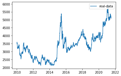
（2）可视化最高价数据

import numpy as np
df_index=df.code
df_index = df_index.index.tolist()
# df_index=[str(year)[0:4] for year in df_index]
df_all = np.array(df['high'].tolist())
df=df['high']
from pandas.plotting import register_matplotlib_converters
import matplotlib.pyplot as plt
register_matplotlib_converters()
# 获取训练数据、原始数据、索引等信息
df, df_all, df_index = readData('high')
#可视化最高价
df_all = np.array(df_all.tolist())
plt.plot(df_index, df_all, label='real-data')
plt.legend(loc='upper right')
<matplotlib.legend.Legend at 0x7fc8a932bfa0>

png

预处理数据

import pandas as pdimport matplotlib.pyplot as pltimport datetimeimport torchimport torch.nn as nnimport numpy as npfrom torch.utils.data import Dataset, DataLoaderimport torchvisionimport torchvision.transforms as transforms%matplotlib inline

（1）生成训练数据

#通过一个序列来生成一个31*(count(*)-train_end)矩阵（用于处理时序的数据）#其中最后一列维标签数据。就是把当天的前n天作为参数，当天的数据作为labeldef generate_data_by_n_days(series, n, index=False): if len(series) <= n: raise Exception("The Length of series is %d, while affect by (n=%d)." % (len(series), n)) df = pd.DataFrame() for i in range(n): df['c%d' % i] = series.tolist()[i:-(n - i)] df['y'] = series.tolist()[n:] if index: df.index = series.index[n:] return df #参数n与上相同。train_end表示的是后面多少个数据作为测试集。def readData(column='high', n=30, all_too=True, index=False, train_end=-500): df = pd.read_csv("sh300.csv", index_col=0) #以日期为索引 df.index = list(map(lambda x: datetime.datetime.strptime(x, "%Y-%m-%d"), df.index)) #获取每天的最高价 df_column = df[column].copy() #拆分为训练集和测试集 df_column_train, df_column_test = df_column[:train_end], df_column[train_end - n:] #生成训练数据 df_generate_train = generate_data_by_n_days(df_column_train, n, index=index) if all_too: return df_generate_train, df_column, df.index.tolist() return df_generate_train

模型

（1）定义模型

class RNN(nn.Module):    def __init__(self, input_size):        super(RNN, self).__init__()        self.rnn = nn.LSTM(            input_size=input_size,            hidden_size=64,            num_layers=1,            batch_first=True        )        self.out = nn.Sequential(            nn.Linear(64, 1)        )    def forward(self, x):        r_out, (h_n, h_c) = self.rnn(x, None)  #None即隐层状态用0初始化 out = self.out(r_out) return outclass mytrainset(Dataset): def __init__(self, data): self.data, self.label = data[:, :-1].float(), data[:, -1].float() def __getitem__(self, index): return self.data[index], self.label[index] def __len__(self): return len(self.data)
（2）超参数设置
n = 30LR = 0.001EPOCH = 200batch_size=20train_end =-600device = torch.device('cuda' if torch.cuda.is_available() else 'cpu')

（3）训练模型

from pandas.plotting import register_matplotlib_convertersregister_matplotlib_converters()# 获取训练数据、原始数据、索引等信息df, df_all, df_index = readData('high', n=n, train_end=train_end)#可视化原高价数据df_all = np.array(df_all.tolist())plt.plot(df_index, df_all, label='real-data')plt.legend(loc='upper right') #对数据进行预处理，规范化及转换为Tensordf_numpy = np.array(df)df_numpy_mean = np.mean(df_numpy)df_numpy_std = np.std(df_numpy)df_numpy = (df_numpy - df_numpy_mean) / df_numpy_stddf_tensor = torch.Tensor(df_numpy)trainset = mytrainset(df_tensor)trainloader = DataLoader(trainset, batch_size=batch_size, shuffle=False)

png

#记录损失值，并用tensorboardx在web上展示
from tensorboardX import SummaryWriter
writer = SummaryWriter(log_dir='logs')
rnn = RNN(n).to(device)
optimizer = torch.optim.Adam(rnn.parameters(), lr=LR)  
loss_func = nn.MSELoss()
for step in range(EPOCH):
    for tx, ty in trainloader:
        tx=tx.to(device)
        ty=ty.to(device)
        #在第1个维度上添加一个维度为1的维度，形状变为[batch,seq_len,input_size]
        output = rnn(torch.unsqueeze(tx, dim=1)).to(device)
        loss = loss_func(torch.squeeze(output), ty)
        optimizer.zero_grad()  
        loss.backward()  
        optimizer.step()
    writer.add_scalar('sh300_loss', loss, step)

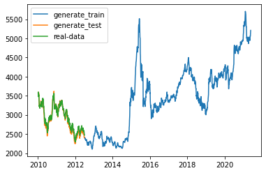
（4）测试模型

generate_data_train = []
generate_data_test = []
test_index = len(df_all) + train_end
df_all_normal = (df_all - df_numpy_mean) / df_numpy_std
df_all_normal_tensor = torch.Tensor(df_all_normal)
for i in range(n, len(df_all)):
    x = df_all_normal_tensor[i - n:i].to(device)
    #rnn的输入必须是3维，故需添加两个1维的维度，最后成为[1,1,input_size]
    x = torch.unsqueeze(torch.unsqueeze(x, dim=0), dim=0)
    y = rnn(x).to(device)
    if i < test_index:
        generate_data_train.append(torch.squeeze(y).detach().cpu().numpy() * df_numpy_std + df_numpy_mean)
    else:
        generate_data_test.append(torch.squeeze(y).detach().cpu().numpy() * df_numpy_std + df_numpy_mean)
plt.plot(df_index[n:train_end], generate_data_train, label='generate_train')
plt.plot(df_index[train_end:], generate_data_test, label='generate_test')
plt.plot(df_index[train_end:], df_all[train_end:], label='real-data')
plt.legend()
plt.show()

png

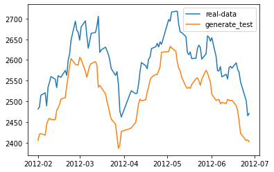
plt.clf()
plt.plot(df_index[train_end:-500], df_all[train_end:-500], label='real-data')
plt.plot(df_index[train_end:-500], generate_data_test[-600:-500], label='generate_test')
plt.legend()
plt.show()