pyTorch代码持续汇总(随机种子-容器-模型初始化-显存回收-数据转换)
1 查询版本信息
import torchprint(torch.__version__) #查看pytorch版本信息print(torch.version.cuda) #查看pytorch所使用的cuda的版本号print(torch.backends.cudnn.version()) #查看pytorch所使用的cudnn的版本号print(torch.cuda.get_device_name(0)) #查看第一块显卡的名称
2 模型训练效果复现
pytoch官方文档:https://pytorch.org/docs/stable/notes/randomness.html
2.1 设置随机种子
随机数是序列,这个序列根据算法计算而来。这个算法有参数,给定一个参数就会产生相应的序列,不同的参数产生不同的序列。不指定随机种子时,将按照一个序列(即默认的某一个参数)依次往下生成随机数,所以每次调用random()都生成不同的随机数。当指定随机数种子时,随机种子的参数确定相应的序列(不指定参数的话还是默认序列),在这个种子作用范围内,调用random()将按照这个序列生成随机数。再次启动程序,即再次进入这个种子时,还按照这个序列从头开始生成随机数。
numpy中seed( )函数用于指定随机数生成时所用算法开始的整数值,需要注意:
- 如果使用相同的seed( )值,则每次生成的随机数都相同;
- 如果不设置这个值,则系统根据时间来自己选择这个值,生成自己的种子,此时每次生成的随机数因时间差异而不同。
- 设置的seed()值仅一次有效。
因此,为了保证在同一台设备上不同次训练的结果可复现,需要设置随机种子为固定值。
import torchimport numpy as npnp.random.seed(0) #设置numpy的随机种子torch.manual_seed(0) #Sets the seed for generating random numberstorch.cuda.manual_seed(0) #Sets the seed for generating random numbers for the current GPU.#It’s safe to call this function if CUDA is not available;#in that case, it is silently ignored.torch.cuda.manual_seed_all(0) #Sets the seed for generating random numbers on all GPUs.
2.2 设置卷积算法
本节内容参考自一篇非常棒的文章:https://blog.csdn.net/byron123456sfsfsfa/article/details/96003317
为了保证结果的可复现性,还应该设置卷积算法相关的参数,具体为:
torch.backends.cudnn.deterministic = Truetorch.backends.cudnn.benchmark = False
下面解释下这两个参数的含义:
cuDNN 是英伟达专门为深度神经网络所开发出来的 GPU 加速库,针对卷积、池化等等常见操作做了非常多的底层优化,比一般的 GPU 程序要快很多。大多数主流深度学习框架都支持 cuDNN,PyTorch 自然也不例外。在使用 GPU 的时候,PyTorch 会默认使用 cuDNN 加速。但是,在使用 cuDNN 的时候,torch.backends.cudnn.benchmark 模式是为 False。所以就意味着,我们的程序有可能还可以继续提速!
如果设置torch.backends.cudnn.benchmark = True,我们就可以在 PyTorch 中对模型里的卷积层进行预先的优化,也就是在每一个卷积层中测试 cuDNN 提供的所有卷积实现算法,然后选择最快的那个。这样在模型启动的时候,只要额外多花一点点预处理时间,就可以较大幅度地减少训练时间。
对应的,设置torch.backends.cudnn.deterministic = True就表示全部用默认的卷积算法,不会为每一个卷积层去找速度最快的实现。
因此,如果为了结果的可复现,就应该设置torch.backends.cudnn.deterministic = True和torch.backends.cudnn.benchmark = False。
2.3 结果可复现的综合实现
参考自:https://zhuanlan.zhihu.com/p/141063432?from_voters_page=true
def init_seeds(seed=0):np.random.seed(seed)torch.manual_seed(seed)torch.cuda.manual_seed(seed)torch.cuda.manual_seed_all(seed)if seed == 0:torch.backends.cudnn.deterministic = Truetorch.backends.cudnn.benchmark = False
3 pyTorch提供的构建网络的容器
pyTorch提供了下述六种容器https://pytorch.org/docs/stable/nn.html#containers。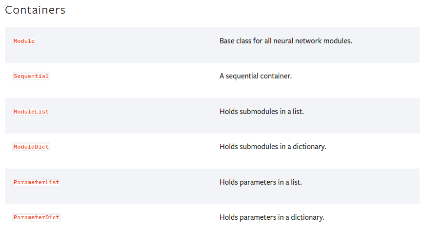
3.1 Module
官方介绍:https://pytorch.org/docs/stable/generated/torch.nn.Module.html#torch.nn.Module
Module是所有神经网络的基类,所有的自定义网络都应该派生自该对象,如下所示:
import torch.nn as nnimport torch.nn.functional as Fclass Model(nn.Module):def __init__(self):super(Model, self).__init__()self.conv1 = nn.Conv2d(1, 20, 5)self.conv2 = nn.Conv2d(20, 20, 5)def forward(self, x):x = F.relu(self.conv1(x))return F.relu(self.conv2(x))
add_module函数用于添加子module;
apply函数用于对module的各子module应用给定的函数,如:
>>> @torch.no_grad()>>> def init_weights(m):>>> print(m)>>> if type(m) == nn.Linear:>>> m.weight.fill_(1.0)>>> print(m.weight)>>> net = nn.Sequential(nn.Linear(2, 2), nn.Linear(2, 2))>>> net.apply(init_weights)
cpu函数将module的所有参数和buffers移动到cpu上;
cuda函数将module的所有参数和buffers移动到GPU上,函数有一个参数,用于指定移动到哪个GPU上。因为优化器也和module的参数进行了关联,所以应该先移动module到gpu上再创建优化器;
3.2 Sequential
Squential是序列化的容器,各子module按照其传入Squential构造函数的顺序进行添加。也可以向构造函数中传入OrderedDict对象。
# Example of using Sequentialmodel = nn.Sequential(nn.Conv2d(1,20,5),nn.ReLU(),nn.Conv2d(20,64,5),nn.ReLU())# Example of using Sequential with OrderedDictmodel = nn.Sequential(OrderedDict([('conv1', nn.Conv2d(1,20,5)),('relu1', nn.ReLU()),('conv2', nn.Conv2d(20,64,5)),('relu2', nn.ReLU())]))class net5(nn.Module):def __init__(self):super(net5,self).__init__()self.block = nn.Sequential(nn.Conv2d(3,32,3),nn.ReLU(),nn.MaxPool2d(2),nn.Conv2d(32,128,3),nn.ReLU(),nn.MaxPool2d(2))def forward(self,x):return self.block(x)net = net5()print(net)
输出:
net5((block): Sequential((0): Conv2d(3, 32, kernel_size=(3, 3), stride=(1, 1))(1): ReLU()(2): MaxPool2d(kernel_size=2, stride=2, padding=0, dilation=1, ceil_mode=False)(3): Conv2d(32, 128, kernel_size=(3, 3), stride=(1, 1))(4): ReLU()(5): MaxPool2d(kernel_size=2, stride=2, padding=0, dilation=1, ceil_mode=False)))
使用nn.Sequential构建的网络,会严格按照构造函数中输入的子module的顺序进行执行。并且自带forward函数,forward过程中会按照子module堆叠的顺序进行运算。
使用OrderedDict对象和nn.Sequential构建的网络,因为输入的是子module名称和对象构成的网络,就是给每一个子module一个自定义的名字。
使用nn.Sequential构建的网络,使用起来方便,不需要自定义forward函数,但也损失了灵活性。
3.3 ModuleList
官方文档:https://pytorch.org/docs/stable/generated/torch.nn.ModuleList.html#torch.nn.ModuleList
ModuleList使用一个list对象hold所有的子module。ModuleList对象可以按照普通list的方式进行索引,但是其包含的子module都会被成功的注册到网络中,子module包含的参数也会自动添加到网络中,调用网络的方法时也会去访问这些子module。对应的,如果使用普通的list来hold所有的子module,这些子module及其参数并不会被注册到网络中,也就无法进行网络的训练。如下面代码对比所示:
class net1(nn.Module):def __init__(self):super(net1,self).__init__()self.linears = nn.ModuleList([nn.Linear(10,10) for i in range(2)])def forward(self,x):for m in self.linears:x = m(x)return xnet = net1()print(net)for name,param in net.named_parameters():print(name,param.shape)class net2(nn.Module):def __init__(self):super(net2,self).__init__()self.linears = [nn.Linear(10,10) for i in range(2)]def forward(self,x):for m in self.linears:x = m(x)return xnet = net2()print(net)print(list(net.parameters()))
输出结果为:
net1((linears): ModuleList((0): Linear(in_features=10, out_features=10, bias=True)(1): Linear(in_features=10, out_features=10, bias=True)))linears.0.weight torch.Size([10, 10])linears.0.bias torch.Size([10])linears.1.weight torch.Size([10, 10])linears.1.bias torch.Size([10])net2()[]
上面的结果可以看出,net1包含网络层和参数,net2的网络层和参数则全部为空。
nn.ModuleList只是保存了已注册到网络中的子module,但并没有设定子module的执行顺序,具体的执行顺序是按照forward函数设定的顺序进行执行的。如下面代码所示:
class net3(nn.Module):def __init__(self):super(net3,self).__init__()self.linears = nn.ModuleList([nn.Linear(10,20),nn.Linear(30,10),nn.Linear(20,30)])def forward(self,x):x = self.linears[0](x)x = self.linears[2](x)x = self.linears[1](x)return xnet = net3()print(net)
另一个细节是,如果对nn.ModuleList中hold的子module在forward函数中进行重复使用,虽然该子module被使用了多次,但其参数却只有一份,相当于在backward过程中进行了多次的参数更新,可能会带来超出预期的训练结果。当然对同一个子module调用多次也没什么特别的用处。
使用nn.ModuleList构建的网络,使用起来略微复杂,需要自己定义forward的顺序,但也带来了灵活性。在重复包含很多相同的网络层的情况下,使用ModuleList是更合适的选择,也可以把各个子module放到一个普通的list对象中,然后使用nn.Sequential(*list)进行解析,如下所示:
class net4(nn.Module):def __init__(self):super(net4,self).__init__()self.linears_list = [nn.Linear(10,10) for i in range(2)]self.linears = nn.Sequential(*self.linears_list)def forward(self,x):x = self.linears_list(x)return xnet = net4()print(net)
输出:
net4((linears): Sequential((0): Linear(in_features=10, out_features=10, bias=True)(1): Linear(in_features=10, out_features=10, bias=True)))
另外,在需要保存网络前向运算中间层结果的时候,如果使用nn.ModuleList,可以在forward函数中将中间层的feature map保存到一个list中返回。如果使用nn.Sequential,则无法使用这种方式,但也可以通过nn.register_forward_hook()实现,相对实现复杂度略高,但forward函数实现更容易。究竟用哪种方式,就看个人喜好了。
特别声明:3.2和3.3节内容参考自:https://blog.csdn.net/byron123456sfsfsfa/article/details/89930990#comments_13093106
3.4 ModuleDict
ModuleDict和ModuleList很像,也是hold网络的子module并将其注册到网络中。区别也就是python中list和dict的区别。
构造ModuleDict对象时传入的是python中的dict对象,可以自定义各子module的名称,如下所示:
class MyModule(nn.Module):def __init__(self):super(MyModule, self).__init__()self.choices = nn.ModuleDict({'conv': nn.Conv2d(10, 10, 3),'pool': nn.MaxPool2d(3)})self.activations = nn.ModuleDict([['lrelu', nn.LeakyReLU()],['prelu', nn.PReLU()]])def forward(self, x, choice, act):x = self.choices[choice](x)x = self.activations[act](x)return x
3.5 ParameterList和ParameterDict
ParameterList和ParameterDict作用是hold网络的参数,并将其注册到网络中。一个是list,一个是dict。
4 模型初始化
官方文档:https://pytorch.org/docs/stable/nn.init.html
4.1 均匀分布:
torch.nn.init.uniform_(tensor, a=0.0, b=1.0)Parameterstensor – an n-dimensional torch.Tensora – the lower bound of the uniform distributionb – the upper bound of the uniform distribution>>> w = torch.empty(3, 5)>>> nn.init.uniform_(w)
4.2 正态分布
生成均值为mean,标注差为std的正态分布。
torch.nn.init.normal_(tensor, mean=0.0, std=1.0)>>> w = torch.empty(3, 5)>>> nn.init.normal_(w)
4.3 常量
torch.nn.init.constant_(tensor, val)
4.4 全1
torch.nn.init.ones_(tensor)
4.5 全0
torch.nn.init.zeros_(tensor)
4.6 对角分布
只针对于二维tensor构建一个对角矩阵
torch.nn.init.eye_(tensor)w = torch.empty(size=(3,5))torch.nn.init.eye_(w)print(w)
输出:
tensor([[1., 0., 0., 0., 0.],[0., 1., 0., 0., 0.],[0., 0., 1., 0., 0.]])
4.7 delta分布
输入tensor为3/4/5维度,产生符合delta分布的输出。
torch.nn.init.dirac_(tensor, groups=1)Parameters:tensor – a {3, 4, 5}-dimensional torch.Tensorgroups (optional) – number of groups in the conv layer (default: 1)
4.8 xavier初始化
4.8.1 xavier
xavier来自于论文《Understanding the difficulty of training deep feedforward neural networks》。
其核心思想是想让神经网络每一层输出的分布都一致。
下面的内容参考自:
https://www.cnblogs.com/hejunlin1992/p/8723816.html
https://blog.csdn.net/ZnZnA/article/details/90081527
预备知识:
假设有两个随机变量w和x,它们都服从均值为0、方差为 σ \sigma σ的随机分布,且独立同分布。那么:
w*x服从均值为0,方差为 σ 2 \sigma ^2 σ2的分布;w*x + w*x服从均值为0,方差为 2 × σ 2 2 \times \sigma ^2 2×σ2的分布。
有了这个预备知识,我们看下,在神经网络中,假设输入数据符合均值为0、方差为 σ \sigma σ的分布,那么经过第一个卷积层进行处理后,得到输出: z = ∑ i = 1 n w i ∗ x i z =\sum_{i=1}^{n}w_i * x_i z=∑i=1nwi∗xi,n = 输入channel数 * 卷积核的宽度 * 卷积核的高度,忽略了偏置项b。
可以看出z符合均值为0、方差为 n × σ x × σ z n \times \sigma_x \times \sigma_z n×σx×σz的分布。如果在层号加到变量的上标处,可以看出:
σ x 2 = n 1 × σ x 1 × σ w 1 \sigma_x^2 = n^1 \times \sigma_x^1 \times \sigma_w^1 σx2=n1×σx1×σw1, σ x 3 = n 2 × σ x 2 × σ w 2 , ⋯ \sigma_x^3 = n^2 \times \sigma_x^2 \times \sigma_w^2,\cdots σx3=n2×σx2×σw2,⋯。那么在第k层,我们有 σ x k = n k − 1 × σ x k − 1 × σ w k − 1 = n k − 1 × n k − 2 × σ x k − 2 × σ w k − 2 × σ w k − 1 \sigma_x^k = n^{k-1} \times \sigma_x^{k-1} \times \sigma_w^{k-1} = n^{k-1} \times n^{k-2} \times \sigma_x^{k-2} \times \sigma_w^{k-2} \times \sigma_w^{k-1} σxk=nk−1×σxk−1×σwk−1=nk−1×nk−2×σxk−2×σwk−2×σwk−1,继续展开,得到 σ x k = σ x 1 Π i = 1 n − 1 n i σ w i \sigma_x^k = \sigma_x^1 \Pi_{i=1}^{n-1} n^i \sigma_w^i σxk=σx1Πi=1n−1niσwi。
从上式可以看出,最后的连乘是很危险的,如果 n i σ w i > 1 n^i \sigma_w^i > 1 niσwi>1,则后面层的方差越来越大;如果 n i σ w i < 1 n^i \sigma_w^i < 1 niσwi<1,则后面层的方差越来越小。
回到出发点来看,作者的目的是为了使各层的方差尽可能保持一致,那么就有 Π i = 1 n − 1 n i σ w i = 1 \Pi_{i=1}^{n-1} n^i \sigma_w^i = 1 Πi=1n−1niσwi=1,即 σ w i = 1 n i \sigma_w^i = \frac{1}{n_i} σwi=ni1,这里的 n i n_i ni表示输入神经元的数量。
上面是从前向传播的角度进行推导的,从方面传播的角度进行推导,可以有相似的结论。
假设我们现在已经得到了输出损失相对于网络第k层的梯度 ∂ l o s s ∂ x k \frac{\partial loss}{\partial x^k} ∂xk∂loss,那么第 k − 1 k-1 k−1层的梯度为 ∂ l o s s ∂ x j k − 1 = ∑ i = 1 n ∂ l o s s ∂ x i k w i j k \frac{\partial loss}{\partial x^{k-1}_j} = \sum_{i=1}^{n}\frac{\partial loss}{\partial x^k_i}w_{ij}^k ∂xjk−1∂loss=∑i=1n∂xik∂losswijk,n表示第k层的神经元的数量。
那么假设最后一层的梯度符合均值为0、方差为某值的分布,那么有: v a r ( ∂ l o s s ∂ x k − 1 ) = n k ∗ v a r ( ∂ l o s s ∂ x k ) ∗ σ w k var(\frac{\partial loss}{\partial x^{k-1}}) = n^k * var(\frac{\partial loss}{\partial x^{k}}) * \sigma_w^k var(∂xk−1∂loss)=nk∗var(∂xk∂loss)∗σwk,对于k层的网络,又推导出公式: v a r ( ∂ l o s s ∂ x 1 ) = v a r ( ∂ l o s s ∂ x k ) ∗ Π i = 1 k − 1 n i ∗ σ w i var(\frac{\partial loss}{\partial x^{1}}) = var(\frac{\partial loss}{\partial x^{k}}) * \Pi_{i=1}^{k-1}n^i * \sigma_w^i var(∂x1∂loss)=var(∂xk∂loss)∗Πi=1k−1ni∗σwi。
上面的连乘,在 n i ∗ σ w i > 1 n^i * \sigma_w^i > 1 ni∗σwi>1时会造成梯度爆炸,在 n i ∗ σ w i < 1 n^i * \sigma_w^i < 1 ni∗σwi<1时会造成梯度弥散。因为为了得到稳定的分布,需要各层的分布尽可能一致,那么就要符合: n i ∗ σ w i = 1 n^i * \sigma_w^i = 1 ni∗σwi=1,即 σ w i = 1 n i \sigma_w^i = \frac{1}{n_i} σwi=ni1,这里的 n i n^i ni表示输出层的神经元数量。
总结,从前向角度看,需要 σ w i = 1 n i \sigma_w^i = \frac{1}{n^i} σwi=ni1,这里的 n i n_i ni表示输入神经元的数量。从反向的角度看,需要 σ w i = 1 n i \sigma_w^i = \frac{1}{n^i} σwi=ni1,这里的 n i n^i ni表示输出层的神经元数量。综合考虑,取两者的调和平均,设置 σ w i = 1 n i + n i + 1 \sigma_w^i = \frac{1}{n^i + n^{i+1}} σwi=ni+ni+11。这个就是xavier初始化的思想。
4.8.2 xavier均匀分布
均匀分布的均值和方差为: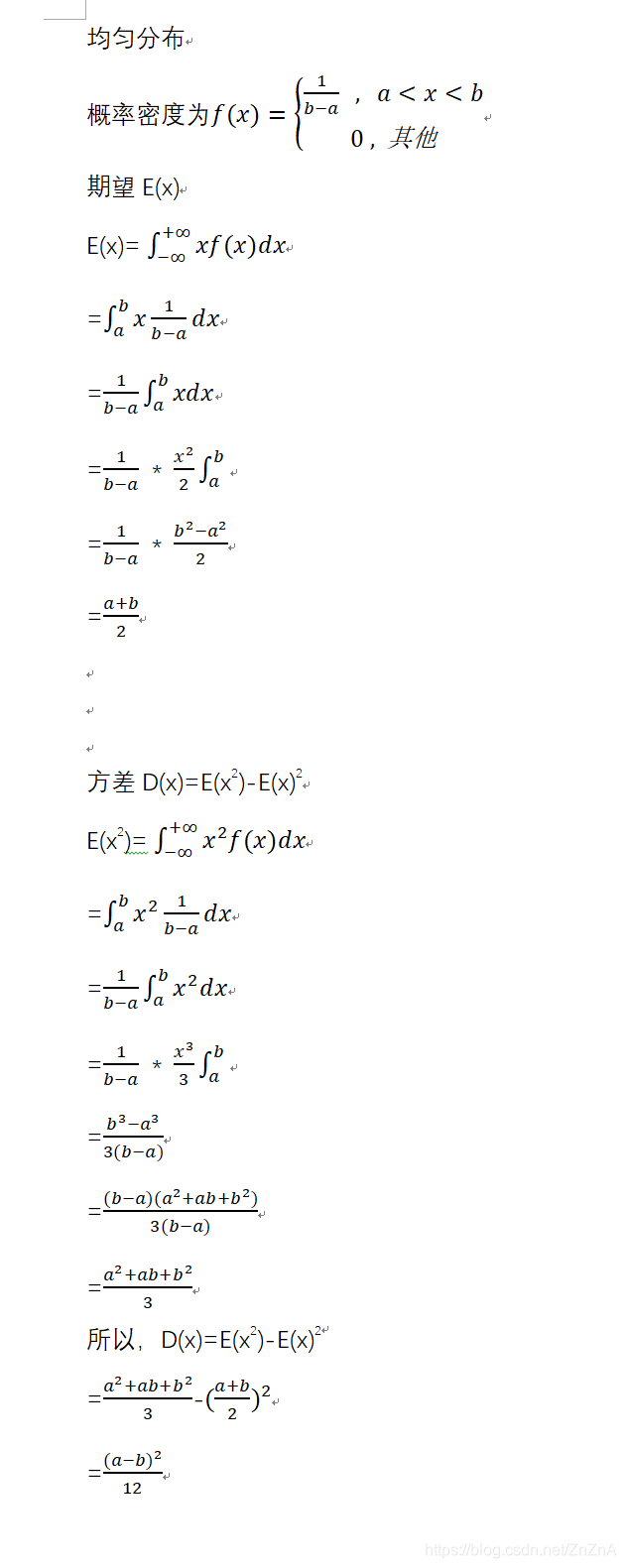
因此,如果我们想得到输出值范围为[-a,a]的均匀分布,那么有: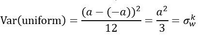
得到: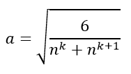
那么xavier均匀分布就是把参数初始化为下面范围内的均匀分布: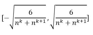
pytorch实现:
torch.nn.init.xavier_uniform_(tensor, gain=1.0)Parameterstensor – an n-dimensional torch.Tensorgain – an optional scaling factor
输出tensor符合取值为[-a,a]的均匀分布,其中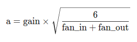
4.8.3 xavier正态分布
torch.nn.init.xavier_normal_(tensor, gain=1.0)Parameterstensor – an n-dimensional torch.Tensorgain – an optional scaling factor
得到符合均值为0、标准差为下式所示的正态分布的输出tensor。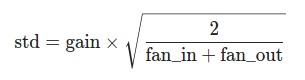
4.9 kaiming初始化
4.9.1 kaiming
来自于论文《Delving deep into rectifiers:Surpassing human-level performance on ImageNet classification》。
kaiming初始化的目的也是为了使网络各层保持相似的分布。
xavier适用于激活函数为sigmoid、tanh时的网络。但在激活函数为Relu函数时,因为负值部分的输入全部被丢掉,只保留了正值部分的输入,那么上面xavier中的推导就不成立了,需要修改为:
前向运算时:
y l = ∑ i = 1 n w l ∗ x l y^l =\sum_{i=1}^{n}w^l * x^{l} yl=∑i=1nwl∗xl,n = 输入channel数 * 卷积核的宽度 * 卷积核的高度,忽略了偏置项b。
因为 x l x^l xl是ReLU函数的输出,其均值不再为0。
作者加强了假设,w不仅独立同分布,均值为0,且为对称分布。由于 x l = R e L U ( y l − 1 ) x^l = ReLU(y^{l-1}) xl=ReLU(yl−1),负半轴产生的方差就不存在了,因此有 v a r ( y l ) = n l ∗ v a r ( w l x l ) = n ∗ v a r ( w l ) ∗ v a r ( x l ) = 1 2 ∗ n l ∗ v a r ( w l ) ∗ v a r ( y l − 1 ) var(y^l) = n^l * var(w^lx^l) = n * var(w^l) * var(x^l) = \frac{1}{2} * n^l * var(w^l) * var(y^{l - 1}) var(yl)=nl∗var(wlxl)=n∗var(wl)∗var(xl)=21∗nl∗var(wl)∗var(yl−1)。
连续堆叠多层,有: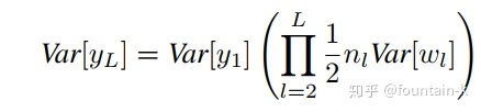
为了保证各层的分布一致,那么就需要保证: 1 2 ∗ n ∗ v a r ( w l ) = 1 \frac{1}{2} * n * var(w^l) = 1 21∗n∗var(wl)=1,即 v a r ( w l ) = 2 n l var(w^l) = \frac{2}{n^l} var(wl)=nl2。
如果使用leaky relu做激活函数时,因为负值部分并未完全清空,其公式为: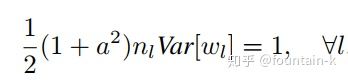
因此, v a r ( w l ) = 2 n l ∗ ( 1 + α 2 ) var(w^l) = \frac{2}{n^l * (1 + \alpha^2)} var(wl)=nl∗(1+α2)2。
4.9.2 kaiming均匀分布
torch.nn.init.kaiming_uniform_(tensor, a=0, mode='fan_in', nonlinearity='leaky_relu')Parameterstensor – an n-dimensional torch.Tensora – the negative slope of the rectifier used after this layer (only used with 'leaky_relu')mode – either 'fan_in' (default) or 'fan_out'. Choosing 'fan_in' preserves the magnitude of the variance of the weights in the forward pass. Choosing 'fan_out' preserves the magnitudes in the backwards pass.nonlinearity – the non-linear function (nn.functional name), recommended to use only with 'relu' or 'leaky_relu' (default).
得到取值范围为[-bound,bound]的均匀分布,其中:
fan_mode在nonlinearity=‘relu’时为 2 n l \frac{2}{n^l} nl2,在nonlinearity=‘leakyrelu’时为 2 n l ∗ ( 1 + α 2 ) \frac{2}{n^l * (1 + \alpha^2)} nl∗(1+α2)2。
4.9.3 kaiming正态分布
torch.nn.init.kaiming_normal_(tensor, a=0, mode='fan_in', nonlinearity='leaky_relu')Parameterstensor – an n-dimensional torch.Tensora – the negative slope of the rectifier used after this layer (only used with 'leaky_relu')mode – either 'fan_in' (default) or 'fan_out'. Choosing 'fan_in' preserves the magnitude of the variance of the weights in the forward pass. Choosing 'fan_out' preserves the magnitudes in the backwards pass.nonlinearity – the non-linear function (nn.functional name), recommended to use only with 'relu' or 'leaky_relu' (default).
输出tensor符合均值为0、标准差如下所示的正态分布: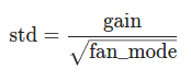
4.10 正交初始化
得到一个正交的或半正交矩阵,输入的tensor大于等于2维。
torch.nn.init.orthogonal_(tensor, gain=1)Parameterstensor – an n-dimensional torch.Tensor, where n≥2n \geq 2n≥2gain – optional scaling factor
4.11 稀疏初始化
torch.nn.init.sparse_(tensor, sparsity, std=0.01)Parameterstensor – an n-dimensional torch.Tensorsparsity – The fraction of elements in each column to be set to zerostd – the standard deviation of the normal distribution used to generate the non-zero values
生成一个稀疏tensor,非零元素采样自均值为0、标准差为std的正态分布。
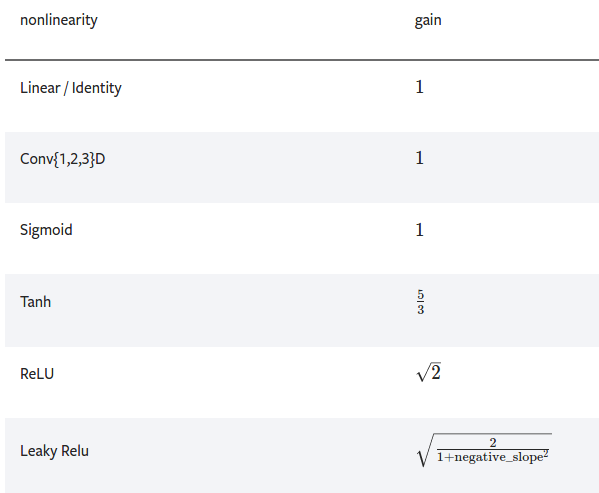
4.12 返回非线性函数的推荐增益值
Gain is a proportional value that shows the relationship between the magnitude of the input to the magnitude of the output signal at the steady state. Many systems contain a method by which the gain can be altered, providing more or less “power” to the system.
torch.nn.init.calculate_gain(nonlinearity, param=None)Parametersnonlinearity – the non-linear function (nn.functional name)param – optional parameter for the non-linear function>>> gain = nn.init.calculate_gain('leaky_relu', 0.2) # leaky_relu with negative_slope=0.2
5 显卡设置及显存回收
设置单张显卡:
device = torch.device('cuda' if torch.cuda.is_available() else 'cpu')
设置多张显卡:
import osos.environ['CUDA_VISIBLE_DEVICES'] = '0,1'
或者在命令行中:
CUDA_VISIBLE_DEVICES=0,1 python train.py
释放显存
torch.cuda.empty_cache()
pyTorch提供了类似于python的存储回收机制,在某块存储区域没有被引用后会自动回收。但是在显存上,每个已经不被占用的显存块不会被立即回收,且在nvidia-smi中查看其仍为占用状态。需要调用
torch.cuda.empty_cache()回收pyTorch已实际未在使用的显存空间,并使其在nvidia-smi中可见。代码验证:
device = torch.device('cuda:0' if torch.cuda.is_available() else 'cpu')dummy_tensor = torch.randn(1200,3,512,512).float().to(device)dummy_tensor = dummy_tensor.to(device='cpu')torch.cuda.empty_cache()
创建
dummy_tensor对象前,显存占用1397MiB;创建后,显存占用5952MiB,理论上应该占用 1200 * 3 * 512 * 512 * 4 / 1024 / 1024大约3700MiB,nvidia-smi查看显存多占用了4500MiB。将dummy_tensor对象移动到内存后,nvidia-smi查看显存仍为5952MiB,表明未占用的显存并未立即回收。调用torch.cuda.empty_cache()后,显存占用变为了2353MiB,回收了不再占用的显存。训练时可以这样使用:
try:output = model(input)except RuntimeError as exception:if "out of memory" in str(exception):print("WARNING: out of memory")if hasattr(torch.cuda, 'empty_cache'):torch.cuda.empty_cache()else:raise exception
参考:https://pytorch.org/docs/stable/notes/cuda.html#cuda-memory-management
https://www.cnblogs.com/jiangkejie/p/11430673.html
https://blog.csdn.net/zxyhhjs2017/article/details/92795831
torch.cuda.get_device_properties(i)获取显卡的属性信息,包括显卡的名称、显存大小等信息。
6 数据类型转换
ndarray和PIL.Image相互转换
image = PIL.Image.fromarray(ndarray.astype(np.uint8))ndarray = np.asarray(PIL.Image.open(path))
ndarray和torch.tensor相互转换
ndarray = tensor.cpu().numpy()tensor = torch.from_numpy(ndarray).float()
torch.tensor和PIL.Image相互转换
# pytorch中的张量默认采用[N, C, H, W]的顺序,并且数据范围在[0,1],需要进行转置和规范化# torch.Tensor -> PIL.Imageimage = PIL.Image.fromarray(torch.clamp(tensor*255, min=0, max=255).byte().permute(1,2,0).cpu().numpy())image = torchvision.transforms.functional.to_pil_image(tensor) # Equivalently way# PIL.Image -> torch.Tensorpath = r'./figure.jpg'tensor = torch.from_numpy(np.asarray(PIL.Image.open(path))).permute(2,0,1).float() / 255tensor = torchvision.transforms.functional.to_tensor(PIL.Image.open(path)) # Equivalently way
参考:https://zhuanlan.zhihu.com/p/104019160


还没有评论,来说两句吧...