《异常检测——从经典算法到深度学习》8 Donut: 基于 VAE 的 Web 应用周期性 KPI 无监督异常检测
《异常检测——从经典算法到深度学习》
- 0 概论
- 1 基于隔离森林的异常检测算法
- 2 基于LOF的异常检测算法
- 3 基于One-Class SVM的异常检测算法
- 4 基于高斯概率密度异常检测算法
- 5 Opprentice——异常检测经典算法最终篇
- 6 基于重构概率的 VAE 异常检测
- 7 基于条件VAE异常检测
- 8 Donut: 基于 VAE 的 Web 应用周期性 KPI 无监督异常检测
- 9 异常检测资料汇总(持续更新&抛砖引玉)
- 10 Bagel: 基于条件 VAE 的鲁棒无监督KPI异常检测
- 11 ADS: 针对大量出现的KPI流快速部署异常检测模型
- 12 Buzz: 对复杂 KPI 基于VAE对抗训练的非监督异常检测
- 13 MAD: 基于GANs的时间序列数据多元异常检测
相关:
- VAE 模型基本原理简单介绍
- GAN 数学原理简单介绍以及代码实践
8. Donut: 基于 VAE 的 Web 应用周期性 KPI 无监督异常检测
2018 Unsupervised Anomaly Detection via Variational Auto-Encoder for Seasonal KPIs in Web Applications
下载地址
8.1 相关资源
8.1.1 论文翻译
为了避免篇幅过长,本文不提供论文翻译部分,如果希望能够读到翻译后的论文的话,请参考本人的个人博客网站 Donut 。
8.1.2 源码地址
这篇论文最大的亮点对于大多数人而言首先就是提供源码,读论文的时候可以找到源码对应地方的实现本身就是非常大的一个亮点。但是并不提供论文使用到的数据集。
源码地址为:https://github.com/NetManAIOps/donut
使用方法也比较简单,需要注意的是,首先确保 tensorflow 版本为 1.x ,如果是 2.x 的话需要重新安装。
8.1.3 源码依赖安装
安装tensorflow 1.15
pip install tensorflow==1.15.4 -i https://pypi.tuna.tsinghua.edu.cn/simple
安装依赖 zhusuan
pip install git+https://github.com/thu-ml/zhusuan.git
安装依赖 tfsnippet
pip install git+https://github.com/haowen-xu/tfsnippet.git@v0.1.2
安装 donut
pip install git+https://github.com/NetManAIOps/donut
如果因为某些原因 clone github 上面的代码比较慢的话,可以考虑克隆到 gitee 上,然后再 clone 并安装。比如说如果租用了某平台的 GPU 。有小伙伴私聊我说了这个事情,我弄了一下这三个地址如下:
- https://gitee.com/smile-yan/zhusuan.git
- https://gitee.com/smile-yan/tfsnippet.git@v0.1.2
- https://gitee.com/smile-yan/donut.git
分别对应上面的github地址。
8.1.4 运行源码注意事项
1 需要注意的是,测试数据总共 5270,然后测试输出数据个数为 5151 。
因为对于每个窗口的检测实际返回的是最后一个窗口的 score,也就是说第一个窗口的前面 119 的点都没有检测,默认为正常数据。因此需要在检测结果前面添加 119 个 0 或者测试数据的真实 label。
2 关于检测结果
并且根据源码对于 get_score 函数的解释,其中提到:
Get the `reconstruction probability` of specified KPI observations.The larger `reconstruction probability`, the less likely a pointis anomaly. You may take the negative of the score, if you wantsomething to directly indicate the severity of anomaly.
这里直接把负数当做异常,处理方法如下:
results = []for temp in test_score:if(temp >= 0):results.append(0)else:results.append(1)
8.2 论文概述
挑选论文几张图片,对论文核心部分进行简单介绍。
8.2.1 时间序列数据集
数据集是单 KPI 时间序列数据,每条数据具有四个属性,KPI,timestamp,value,label。比如说:
| timestamp | value | label | |
|---|---|---|---|
| 0 | 1469376000 | 0.847300 | 0 |
| 1 | 1469376300 | -0.036137 | 0 |
| 2 | 1469376600 | 0.074292 | 0 |
| 3 | 1469376900 | 0.074292 | 0 |
| 4 | 1469377200 | -0.036137 | 0 |
| … | … | … | … |
但是论文具体用的是什么时间序列数据集并不清楚。
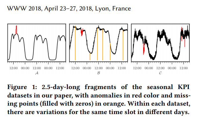
另外注意论文提到的数据的特点,如下图所示: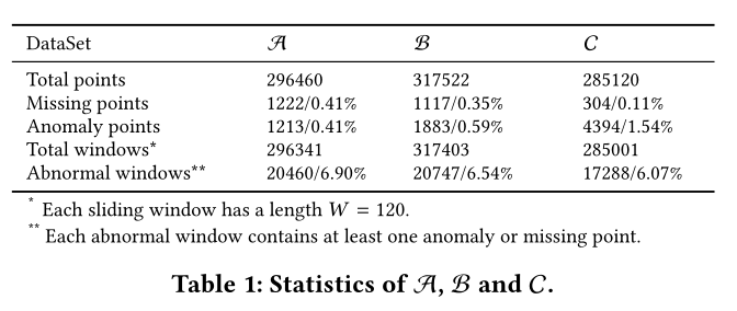
8.2.2 Donut 结构
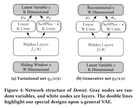
相对于 VAE, Donut 把两个网络拆开展示,并且针对于时间序列数据使用了滑动窗口将序列数据转换成多组数据。然后根据把整个窗口数据进行重构。
8.2.3 缺失数据填充

论文使用 MCMC 与 已进训练的 VAE 进行缺失数据填充,具体操作可以参考后面的内容。
8.2.4 对比实验
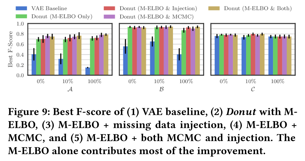
这些实验都使用了 VAE 、滑动窗口 与 重构概率。然后再添加其他技术,进行实验对比。值得一提的是,如果希望做这些对比实验的话,可以对 Donut 源码进行修改。
M-ELBO 对 VAE-baseline 的大部分改善作了贡献。它通过训练 Donut 来适应 x x x 中可能的异常点,并在这种情况下产生期望的输出。虽然我们期望 M-ELBO 能够发挥作用,但我们并没有期望它能发挥这么好的作用。总之,虽然对于生成模型来说这是很自然的,但是仅仅使用正常数据来训练V AE进行异常检测并不是一个好的做法(§5.2)。据我们所知,M-ELBO 及其重要性在以前的工作中从未提到过,因此是我们的一项重大贡献。
Missing data injection (缺失的数据注入)是为了提高 M-ELBO 的效果而设计的,实际上也可以看作数据优化的一种方法。事实上,如果我们在训练时同时注入缺失数据和综合生成的异常数据,那效果将会更好。然而,生成与真实异常数据足够相似的数据比较困难,这应该是一个大主题,超出了本文的涉及范围。因此,我们只是注入缺失的点。缺失数据的注入对最优F-score的提高不是很明显,并且当 B , C \mathcal{B,C} B,C 无标注时,效果只比只使用 M-ELBO 差一点点。这可能是因为注入给训练带来了额外的随机性,因此它需要更大的训练周期,与M-ELBO的情况相比。我们不确定在采用注入时要运行多少个epoch,为了得到一个客观的比较,因此我们在所有情况下都使用相同的epoch,而保持结果不变。我们仍然建议使用缺失数据注入,即使要花费更大的训练周期,因为它预计有很大的工作机会。
MCMC imputation 也被设计用来帮助 Donut 处理异常点。虽然只是在一些情况下 Donut 通过使用 MCMC 让 F-score 值得到了很大的优化,但是它绝对不会降低检测结果。根据文献[32],这应该是预期的结果。 因此,我们建议在检测中始终采用 MCMC。
8.3 论文与源码
本部分将结合源码进行分析论文。
8.3.1 损失函数
论文提出了不同于标准的 ELBO 的损失函数。
VAE 的标准损失函数 ELBO 公式如下: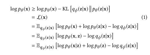
而本文提出来的计算损失的函数公式为: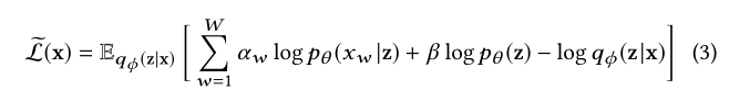
论文对此的解释在 3.2 节,总共有两个参数 α \alpha α 与 β \beta β , 为指示符, α w = 1 \alpha_w = 1 αw=1 表明 x w x_w xw 不是异常,也不是缺失值。 β \beta β 被定义为 ( ∑ w = 1 W α w ) / W (\sum_{w=1}^{W}\alpha_w)/W (∑w=1Wαw)/W。通过 α w \alpha_w αw 去除标记为异常或缺失值的 p θ ( x w ∣ z ) p_\theta{(x_w|z)} pθ(xw∣z) 的影响,然后缩放因子 β \beta β 根据 x x x 中正常点所占的比重缩小 p θ ( z ) p_\theta{(z)} pθ(z) 的贡献。
对应的源码部分在 model.py 文件中,具体地址为 https://github.com/NetManAIOps/donut/blob/master/donut/model.py
def get_training_loss(self, x, y, n_z=None):""" Get the training loss for `x` and `y`. Args: x (tf.Tensor): 2-D `float32` :class:`tf.Tensor`, the windows of KPI observations in a mini-batch. y (tf.Tensor): 2-D `int32` :class:`tf.Tensor`, the windows of ``(label | missing)`` in a mini-batch. n_z (int or None): Number of `z` samples to take for each `x`. (default :obj:`None`, one sample without explicit sampling dimension) Returns: tf.Tensor: 0-d tensor, the training loss, which can be optimized by gradient descent algorithms. """with tf.name_scope('Donut.training_loss'):chain = self.vae.chain(x, n_z=n_z)x_log_prob = chain.model['x'].log_prob(group_ndims=0)alpha = tf.cast(1 - y, dtype=tf.float32)beta = tf.reduce_mean(alpha, axis=-1)log_joint = (tf.reduce_sum(alpha * x_log_prob, axis=-1) +beta * chain.model['z'].log_prob())vi = VariationalInference(log_joint=log_joint,latent_log_probs=chain.vi.latent_log_probs,axis=chain.vi.axis)loss = tf.reduce_mean(vi.training.sgvb())return loss
其中,alpha 的计算就是得到 [0. 1. 0. 1. 1.] 这样的数列。
然后 tf.reduce_mean 用来计算异常的比重。beta 等于这个比重。特别值得一提的是,如果是无监督学习的话,也就是说把所有的 labels 设置为 0 的时候,那么很明显此时的代码中的 y = [0 0 …],此时的 α \alpha α=[1,1,1,1…],而 β \beta β也等于1,也就是说,如果是无监督学习的话,那么整个 M-ELBO 就等于VAE的标准 ELBO。
另外特别需要注意的,如同源码注释一样,函数参数 x x x 是一个二维数据,因为是一个 mini-batch 的训练方法,每次传入的数据都是若干批次数据,比如说如果每个批次传入 32 条数据,也就是 32 个窗口数据并且窗口大小为 120 的话,那么输入的 x x x 的 shape 为 (32, 120)。当然,同样地,返回结果也是 32 组数据。
8.3.2 缺失数据填充
Donut 对数据的预处理包括两方面,一个是对 KPI value 的标准化,另外一个是缺失数据填充。都可以在 preprocessing.py 文件中找到源码。
缺失数据填充包括两部分,一个是时间戳,一个是 values。首先填充时间戳是非常容易的,根据顺序填充即可。而 values 的填充论文在 3.3 节解释了——即 基于 MCMC 和训练好的 VAE 的缺失数据填充技术 。关于这个技术的代码在后面重构概率的计算中介绍。
8.3.3 重构概率计算
重构概率计算关系到如何判定异常,或者说给数据进行异常值打分,然后再根据设定好的阈值判定异常。
1 首先查看一下 donut 的使用方法 源码。
from donut import DonutTrainer, DonutPredictortrainer = DonutTrainer(model=model, model_vs=model_vs)predictor = DonutPredictor(model)with tf.Session().as_default():trainer.fit(train_values, train_labels, train_missing, mean, std)test_score = predictor.get_score(test_values, test_missing)
特别关注最后一行,test_score = predictor.get_score(test_values, test_missing).
查看 model.py 文件,查看其中的 get_score 函数。
2 接着查看donut 的 prediction.py 文件,这里的 get_score 函数直接用于计算异常值。
def get_score(self, values, missing=None):""" Get the `reconstruction probability` of specified KPI observations. The larger `reconstruction probability`, the less likely a point is anomaly. You may take the negative of the score, if you want something to directly indicate the severity of anomaly. Args: values (np.ndarray): 1-D float32 array, the KPI observations. missing (np.ndarray): 1-D int32 array, the indicator of missing points. If :obj:`None`, the MCMC missing data imputation will be disabled. (default :obj:`None`) Returns: np.ndarray: The `reconstruction probability`, 1-D array if `last_point_only` is :obj:`True`, or 2-D array if `last_point_only` is :obj:`False`. """with tf.name_scope('DonutPredictor.get_score'):sess = get_default_session_or_error()collector = []# validate the argumentsvalues = np.asarray(values, dtype=np.float32)if len(values.shape) != 1:raise ValueError('`values` must be a 1-D array')# run the prediction in mini-batchessliding_window = BatchSlidingWindow(array_size=len(values),window_size=self.model.x_dims,batch_size=self._batch_size,)if missing is not None:missing = np.asarray(missing, dtype=np.int32)if missing.shape != values.shape:raise ValueError('The shape of `missing` does not agree ''with the shape of `values` ({} vs {})'.format(missing.shape, values.shape))for b_x, b_y in sliding_window.get_iterator([values, missing]):feed_dict = dict(six.iteritems(self._feed_dict))feed_dict[self._input_x] = b_xfeed_dict[self._input_y] = b_yb_r = sess.run(self._get_score(), feed_dict=feed_dict)collector.append(b_r)else:for b_x, in sliding_window.get_iterator([values]):feed_dict = dict(six.iteritems(self._feed_dict))feed_dict[self._input_x] = b_xb_r = sess.run(self._get_score_without_y(),feed_dict=feed_dict)collector.append(b_r)# merge the results of mini-batchesresult = np.concatenate(collector, axis=0)return result
需要注意的是,当查看源码的时候,发现其真真正正用于计算每个窗口数据的重构概率的也并不在这个文件中,而是在 model.py 文件中。这里只是对流数据进行窗口化处理。
3 查看 model.py 文件,关注其中的 get_score 函数。函数用于计算单个窗口的重构概率,可以选择返回窗口中每个数据的重构概率,也可以选择返回窗口中最后一个点的重构概率。
这个作为重中之重,我添加了一些注释。
def get_score(self, x, y=None, n_z=None, mcmc_iteration=None,last_point_only=True):""" Get the reconstruction probability for `x` and `y`. The larger `reconstruction probability`, the less likely a point is anomaly. You may take the negative of the score, if you want something to directly indicate the severity of anomaly. Args: x (tf.Tensor): 2-D `float32` :class:`tf.Tensor`, the windows of KPI observations in a mini-batch. y (tf.Tensor): 2-D `int32` :class:`tf.Tensor`, the windows of missing point indicators in a mini-batch. n_z (int or None): Number of `z` samples to take for each `x`. (default :obj:`None`, one sample without explicit sampling dimension) mcmc_iteration (int or tf.Tensor): Iteration count for MCMC missing data imputation. (default :obj:`None`, no iteration) last_point_only (bool): Whether to obtain the reconstruction probability of only the last point in each window? (default :obj:`True`) Returns: tf.Tensor: The reconstruction probability, with the shape ``(len(x) - self.x_dims + 1,)`` if `last_point_only` is :obj:`True`, or ``(len(x) - self.x_dims + 1, self.x_dims)`` if `last_point_only` is :obj:`False`. This is because the first ``self.x_dims - 1`` points are not the last point of any window. """with tf.name_scope('Donut.get_score'):# MCMC missing data imputation## 如果存在缺失值,并且选择使用 mcmc 填充## x_r 即对数据 x 的重构数据if y is not None and mcmc_iteration:x_r = iterative_masked_reconstruct(reconstruct=self.vae.reconstruct,x=x,mask=y,iter_count=mcmc_iteration,back_prop=False,)else:x_r = x# get the reconstruction probability## 传入 x_r 到 变分网络 q_netq_net = self.vae.variational(x=x_r, n_z=n_z) # notice: x=x_r## 传入隐变量 z 和 x 到生成网络 p_netp_net = self.vae.model(z=q_net['z'], x=x, n_z=n_z) # notice: x=x# 计算重构概率r_prob = p_net['x'].log_prob(group_ndims=0)if n_z is not None:n_z = validate_n_samples(n_z, 'n_z')assert_shape_op = tf.assert_equal(tf.shape(r_prob),tf.stack([n_z, tf.shape(x)[0], self.x_dims]),message='Unexpected shape of reconstruction prob')with tf.control_dependencies([assert_shape_op]):r_prob = tf.reduce_mean(r_prob, axis=0)if last_point_only:r_prob = r_prob[:, -1]return r_prob
4 最后看一下重构函数,也就是 reconstruction.py 文件,这个文件其他地方都比较容易理解,重点关注最后的几行。
其中的 iter_count 是传入的整数,迭代次数,masked_reconstruct 是定义在该 py 文件的函数,
# do the masked reconstructionsx_r, _ = tf.while_loop(lambda x_i, i: i < iter_count,lambda x_i, i: (masked_reconstruct(reconstruct, x_i, mask), i + 1),[x, tf.constant(0, dtype=tf.int32)],back_prop=back_prop)
可以把那两行 lambda 理解为:
while(i < iter_count):x_i = masked_reconstruct(reconstruct, x_i, mask)i = i + 1return x_i,i
tf.while_loop 执行的也就是上面的这些代码的意思。
8.3.4 训练
训练相关代码都在 training.py 文件中,内容比较多,这里不附加所有源码了,请自行查看。
特别需要介绍的是这个 DonutTrainer 类的参数,因为在实际使用的时候可以考虑调参优化的时候,可以参考这些内容。
model:比如Donut模型,总之是训练对象,是一种 VAE 模型。model_vs:其中的vs可以认为是variables space的缩写,即模型相关的可优化参数空间。如果指定了,将会只在这个空间内收集可优化参数;如果为空的话,将会收集训练过程中所有的可优化参数。n_z:即Donut模型隐变量的个数。
8.4 论文勘误
论文存在几个小小问题,当然,也有可能是因为我是从 arxiv 网站上下载的有关,论文中提到的图片与实际图片不符。在 4.5 节的时候,提到的 图9 和 图10 弄反了。
8.5 总结
论文还有更多内容这里都没有提到,希望伙伴们都可以去看一下。这里主要是基于源码进行简单的分析,把最容易困扰的地方说明一下,既作为自己论文阅读与实验的笔记,也希望能帮助到更多人。如果有任何疑问或者觉得本文应该补充的地方,请留言说明,感谢!
Smileyan
2021.1.10 21:50
最后更新:2021.1.28 10:41
感谢您的 点赞、 收藏、评论 与 关注


")
")
AxureRP8基础操作")
集成jedis访问redis集群")


还没有评论,来说两句吧...