Assigment1 k-Nearest Neighbor (kNN) exercise (1)
Assigment1 k-Nearest Neighbor (kNN) exercise (1)
一、作业内容
- (感觉很多深度学习相关课程的入门第一课都是kNN啊。。。可能是因为它具有提高学习兴趣的魔力?或者比较简单??)kNN分类器是一种十分简单暴力的分类器,算法原理简单易懂,就是计算距离以进行比较,它包含两个主要步骤:
1)训练
- 这里的训练应该加上下引号,因为它其实啥也没干,仅仅读取了训练数据并进行存储以供后续调用
2)测试
- 对于每一个测试样本,此课程即为测试图像,kNN将遍历一次训练集合,计算该测试图像与训练集中每一张图像的距离(暴力之处),通过排序等方法找出距离最近的k张图像,在这k张图像中,占多数的标签类别就是该测试图像所属的类别
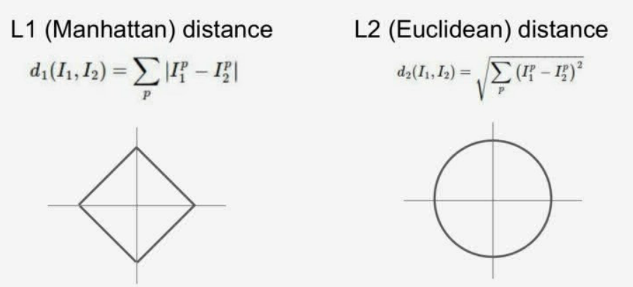
而计算图像的距离主要有两种方式,分别是曼哈顿距离(L1距离)和欧几里得距离(L2距离),具体差别如下图所示:
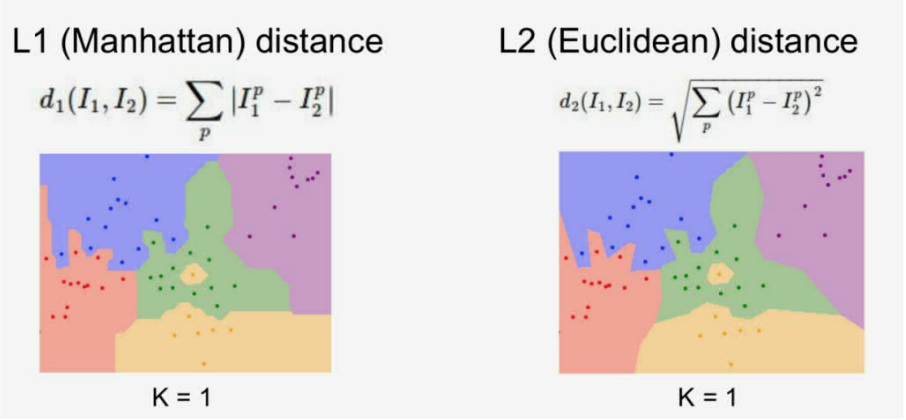
课程中针对这两种距离计算方法进行了可视化比较,如下图所示。但是具体使用哪种距离度量就要视情况而定了,我们可以通过具体场景下的效果对比来进行探索
二、完成作业
- 港真,我觉得这课的课程机制真滴好,作业的格式安排简直人性化,不会让人走弯路的感觉(个人感受)。基本上,学生要完成的工作都在py文件里,而且是通过完善函数功能的方式。然后他的notebook中已经有很多的预备代码,调用那些py文件来训练模型、测试数据等,而且notebook中还包含了大部分的说明,感觉做作业的过程是种享受。。。
废话不多说,接下来就开始记录我的完成过程。首先跑一下notebook中的setup代码,主要是几个基本的配置
Run some setup code for this notebook.
import random
import numpy as np
from cs231n.data_utils import load_CIFAR10
import matplotlib.pyplot as pltThis is a bit of magic to make matplotlib figures appear inline in the notebook
rather than in a new window.
%matplotlib inline
plt.rcParams[‘figure.figsize’] = (10.0, 8.0) # set default size of plots
plt.rcParams[‘image.interpolation’] = ‘nearest’
plt.rcParams[‘image.cmap’] = ‘gray’Some more magic so that the notebook will reload external python modules;
see http://stackoverflow.com/questions/1907993/autoreload-of-modules-in-ipython
%load_ext autoreload
%autoreload 2接下来就是加载数据,包括训练数据和测试数据(均分为X部分和Y部分)
Load the raw CIFAR-10 data.
cifar10_dir = ‘cs231n/datasets/cifar-10-batches-py’
Cleaning up variables to prevent loading data multiple times (which may cause memory issue)
try:
del X_train, y_train
del X_test, y_test
print(‘Clear previously loaded data.’)
except:
passX_train, y_train, X_test, y_test = load_CIFAR10(cifar10_dir)
As a sanity check, we print out the size of the training and test data.
print(‘Training data shape: ‘, X_train.shape)
print(‘Training labels shape: ‘, y_train.shape)
print(‘Test data shape: ‘, X_test.shape)
print(‘Test labels shape: ‘, y_test.shape)可以看到上述代码进行了输出,主要是输出了数据的shape,如下所示
Training data shape: (50000, 32, 32, 3)
Training labels shape: (50000,)
Test data shape: (10000, 32, 32, 3)
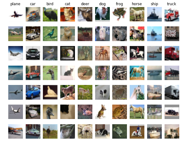
Test labels shape: (10000,)可能还对这一套数据集不熟悉?这里就将数据集中每一类的样本都随机挑选几个进行展示,代码如下:
Visualize some examples from the dataset.
We show a few examples of training images from each class.
classes = [‘plane’, ‘car’, ‘bird’, ‘cat’, ‘deer’, ‘dog’, ‘frog’, ‘horse’, ‘ship’, ‘truck’]
num_classes = len(classes)
samples_per_class = 7
for y, cls in enumerate(classes):idxs = np.flatnonzero(y_train == y)idxs = np.random.choice(idxs, samples_per_class, replace=False)for i, idx in enumerate(idxs):plt_idx = i * num_classes + y + 1plt.subplot(samples_per_class, num_classes, plt_idx)plt.imshow(X_train[idx].astype('uint8'))plt.axis('off')if i == 0:plt.title(cls)
plt.show()
上述代码中有个函数值得一提,即 numpy.flatnonzero() 。其最基本的功能就是输入一个矩阵,返回矩阵中非零元素的位置,如下所示:
x = np.arange(-2, 3)
x
array([-2, -1, 0, 1, 2])
np.flatnonzero(x)
array([0, 1, 3, 4])
import numpy as npd = np.array([1,2,3,4,4,3,5,3,6])tmp = np.flatnonzero(d == 3)print(tmp)[2 5 7]
- 观察上述代码中的tmp,你就能get到 idxs = np.flatnonzero(y_train == y) 这一行代码的作用,它找出了标签中y类的位置。执行这一段可视化代码的结果如下:
整个数据集比较大,kNN又比较暴力,所以仅取一个子集来进行练习,代码如下
Subsample the data for more efficient code execution in this exercise
num_training = 5000
mask = list(range(num_training))
X_train = X_train[mask]
y_train = y_train[mask]num_test = 500
mask = list(range(num_test))
X_test = X_test[mask]
y_test = y_test[mask]Reshape the image data into rows
X_train = np.reshape(X_train, (X_train.shape[0], -1))
X_test = np.reshape(X_test, (X_test.shape[0], -1))
print(X_train.shape, X_test.shape)接下来就要创建kNN分类器了(其实只是对训练数据进行了简单存储)。我们要做的工作主要是计算距离矩阵,如果训练样本有 N t r Ntr Ntr 个,测试样本有 N t e Nte Nte 个,则距离矩阵应该是个 N t r ∗ N t e Ntr * Nte Ntr∗Nte 大小的矩阵,其中元素 [i, j] 表示第 i 个测试样本到第 j 个训练样本的距离。接下来,就是补全 k_nearest_neighbor.py 文件中的 compute_distances_two_loops 方法,它使用粗暴的两层循环来计算测试样本与训练样本之间的距离
def compute_distances_two_loops(self, X):
""" Compute the distance between each test point in X and each training point in self.X_train using a nested loop over both the training data and the test data. Inputs: - X: A numpy array of shape (num_test, D) containing test data. Returns: - dists: A numpy array of shape (num_test, num_train) where dists[i, j] is the Euclidean distance between the ith test point and the jth training point. """num_test = X.shape[0]num_train = self.X_train.shape[0]dists = np.zeros((num_test, num_train))for i in range(num_test):for j in range(num_train):###################################################################### TODO: ## Compute the l2 distance between the ith test point and the jth ## training point, and store the result in dists[i, j]. You should ## not use a loop over dimension, nor use np.linalg.norm(). ####################################################################### *****START OF YOUR CODE (DO NOT DELETE/MODIFY THIS LINE)*****dists[i][j] = np.sqrt(np.sum(np.square(X[i,:] - self.X_train[j,:])))# *****END OF YOUR CODE (DO NOT DELETE/MODIFY THIS LINE)*****return dists
作业中还要求测试上述方法,并进行了可视化,但我觉得意义不大,这里就不做记录了。直接跳到下一个步骤,实现 predict_labels 方法,以结合 compute_distances_two_loops 方法进行测试样本分类
def predict_labels(self, dists, k=1):
""" Given a matrix of distances between test points and training points, predict a label for each test point. Inputs: - dists: A numpy array of shape (num_test, num_train) where dists[i, j] gives the distance betwen the ith test point and the jth training point. Returns: - y: A numpy array of shape (num_test,) containing predicted labels for the test data, where y[i] is the predicted label for the test point X[i]. """num_test = dists.shape[0]y_pred = np.zeros(num_test)for i in range(num_test):# A list of length k storing the labels of the k nearest neighbors to# the ith test point.closest_y = []########################################################################## TODO: ## Use the distance matrix to find the k nearest neighbors of the ith ## testing point, and use self.y_train to find the labels of these ## neighbors. Store these labels in closest_y. ## Hint: Look up the function numpy.argsort. ########################################################################### *****START OF YOUR CODE (DO NOT DELETE/MODIFY THIS LINE)*****closest_y = self.y_train[np.argsort(dists[i])[:k]]# *****END OF YOUR CODE (DO NOT DELETE/MODIFY THIS LINE)*****########################################################################## TODO: ## Now that you have found the labels of the k nearest neighbors, you ## need to find the most common label in the list closest_y of labels. ## Store this label in y_pred[i]. Break ties by choosing the smaller ## label. ########################################################################### *****START OF YOUR CODE (DO NOT DELETE/MODIFY THIS LINE)*****y_pred[i] = np.argmax(np.bincount(closest_y))# *****END OF YOUR CODE (DO NOT DELETE/MODIFY THIS LINE)*****return y_pred
值得一提的是 numpy.bincount 函数,这里需要记录前k个训练样本中没中类别出现的次数,而 numpy.bincount 函数就能优雅的完成这一任务,下面给出两个例子你就懂了:
我们可以看到x中最大的数为7,因此bin的数量为8,那么它的索引值为0->7
x = np.array([0, 1, 1, 3, 2, 1, 7])
索引0出现了1次,索引1出现了3次……索引5出现了0次……
np.bincount(x)
因此,输出结果为:array([1, 3, 1, 1, 0, 0, 0, 1])
我们可以看到x中最大的数为7,因此bin的数量为8,那么它的索引值为0->7
x = np.array([7, 6, 2, 1, 4])
索引0出现了0次,索引1出现了1次……索引5出现了0次……
np.bincount(x)
输出结果为:array([0, 1, 1, 0, 1, 0, 1, 1])
进行测试并计算准确率,首先取 k=1
Now implement the function predict_labels and run the code below:
We use k = 1 (which is Nearest Neighbor).
y_test_pred = classifier.predict_labels(dists, k=1)
Compute and print the fraction of correctly predicted examples
num_correct = np.sum(y_test_pred == y_test)
accuracy = float(num_correct) / num_test
print(‘Got %d / %d correct => accuracy: %f’ % (num_correct, num_test, accuracy))输出准确率
Got 137 / 500 correct => accuracy: 0.274000
取 k=5
y_test_pred = classifier.predict_labels(dists, k=5)
num_correct = np.sum(y_test_pred == y_test)
accuracy = float(num_correct) / num_test
print(‘Got %d / %d correct => accuracy: %f’ % (num_correct, num_test, accuracy))输出准确率
Got 139 / 500 correct => accuracy: 0.278000
可以看到k取5的效果会优于k取1,但这是随意取的,后续会使用交叉验证的方法来选择最优的超参数k,在下一篇博客进行记录吧
接下来要将距离计算的效率提升一下,使用单层循环结构的计算方法,需要补全 compute_distances_one_loop 方法,主要是利用了广播机制,减少了一层循环
def compute_distances_one_loop(self, X):
""" Compute the distance between each test point in X and each training point in self.X_train using a single loop over the test data. Input / Output: Same as compute_distances_two_loops """num_test = X.shape[0]num_train = self.X_train.shape[0]dists = np.zeros((num_test, num_train))for i in range(num_test):######################################################################## TODO: ## Compute the l2 distance between the ith test point and all training ## points, and store the result in dists[i, :]. ## Do not use np.linalg.norm(). ######################################################################### *****START OF YOUR CODE (DO NOT DELETE/MODIFY THIS LINE)*****# 利用broadcasting,一次性算出每一张图片与5000张图片的距离dists[i, :] = np.sqrt(np.sum(np.square(self.X_train - X[i, :]),axis=1))# *****END OF YOUR CODE (DO NOT DELETE/MODIFY THIS LINE)*****return dists
还能继续优化吗?能!通过矩阵乘法和两次广播加法,可以不使用循环,就能完成计算任务
def compute_distances_no_loops(self, X):
""" Compute the distance between each test point in X and each training point in self.X_train using no explicit loops. Input / Output: Same as compute_distances_two_loops """num_test = X.shape[0]num_train = self.X_train.shape[0]dists = np.zeros((num_test, num_train))########################################################################## TODO: ## Compute the l2 distance between all test points and all training ## points without using any explicit loops, and store the result in ## dists. ## ## You should implement this function using only basic array operations; ## in particular you should not use functions from scipy, ## nor use np.linalg.norm(). ## ## HINT: Try to formulate the l2 distance using matrix multiplication ## and two broadcast sums. ########################################################################### *****START OF YOUR CODE (DO NOT DELETE/MODIFY THIS LINE)*****def compute_distances_no_loops(self, X):""" Compute the distance between each test point in X and each training point in self.X_train using no explicit loops. Input / Output: Same as compute_distances_two_loops """num_test = X.shape[0]num_train = self.X_train.shape[0]dists = np.zeros((num_test, num_train))########################################################################## TODO: ## Compute the l2 distance between all test points and all training ## points without using any explicit loops, and store the result in ## dists. ## ## You should implement this function using only basic array operations; ## in particular you should not use functions from scipy, ## nor use np.linalg.norm(). ## ## HINT: Try to formulate the l2 distance using matrix multiplication ## and two broadcast sums. ########################################################################### *****START OF YOUR CODE (DO NOT DELETE/MODIFY THIS LINE)*****temp_2xy = np.dot(X,self.X_train.T) * (-2)temp_x2 = np.sum(np.square(X),axis=1,keepdims=True)temp_y2 = np.sum(np.square(self.X_train),axis=1)dists = temp_x2 + temp_2xy + temp_y2# 上述四行的作用,构造出了 x^2-2xy+y^2# 然后开根号即可dists = np.sqrt(dists)# *****END OF YOUR CODE (DO NOT DELETE/MODIFY THIS LINE)*****return dists# *****END OF YOUR CODE (DO NOT DELETE/MODIFY THIS LINE)*****return dists
这三个计算距离的函数所计算出的结果都是一样的,就不再赘述了,主要是比较一下他们的效率
Let’s compare how fast the implementations are
def time_function(f, *args):
""" Call a function f with args and return the time (in seconds) that it took to execute. """import timetic = time.time()f(*args)toc = time.time()return toc - tic
two_loop_time = time_function(classifier.compute_distances_two_loops, X_test)
print(‘Two loop version took %f seconds’ % two_loop_time)one_loop_time = time_function(classifier.compute_distances_one_loop, X_test)
print(‘One loop version took %f seconds’ % one_loop_time)no_loop_time = time_function(classifier.compute_distances_no_loops, X_test)
print(‘No loop version took %f seconds’ % no_loop_time)输出如下,可以很明显地看到效率差距
Two loop version took 47.337988 seconds
One loop version took 45.795947 seconds
No loop version took 0.334743 seconds


")


还没有评论,来说两句吧...