理解 TensorFlow 之 word2vec

自然语言处理（英语：Natural Language Processing，简称NLP）是人工智能和语言学领域的分支学科。自然语言生成系统把计算机数据转化为自然语言。自然语言理解系统把自然语言转化为计算机程序更易于处理的形式。

一般，计算机要处理文本，需要先把文本向量化，即把文本映射到向量空间模型中，再应用深度学习方法来训练。

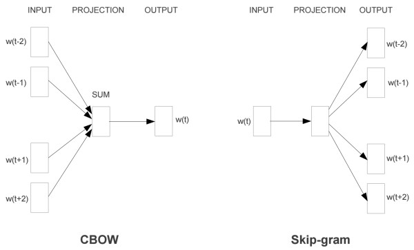
Word2vec 是一种可以进行高效率词嵌套学习的预测模型。其两种变体分别为：连续词袋模型（CBOW）及Skip-Gram模型

回想一下多层感知器训练 mnist 数据集的例子

TensorFlow MNIST机器学习入门

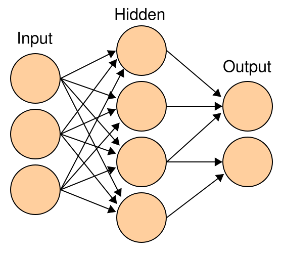
每个输入的图片数据是一个 784 维的向量

对于softmax回归模型可以用下面的图解释，对于输入的xs加权求和，再分别加上一个偏置量，最后再输入到softmax函数中：

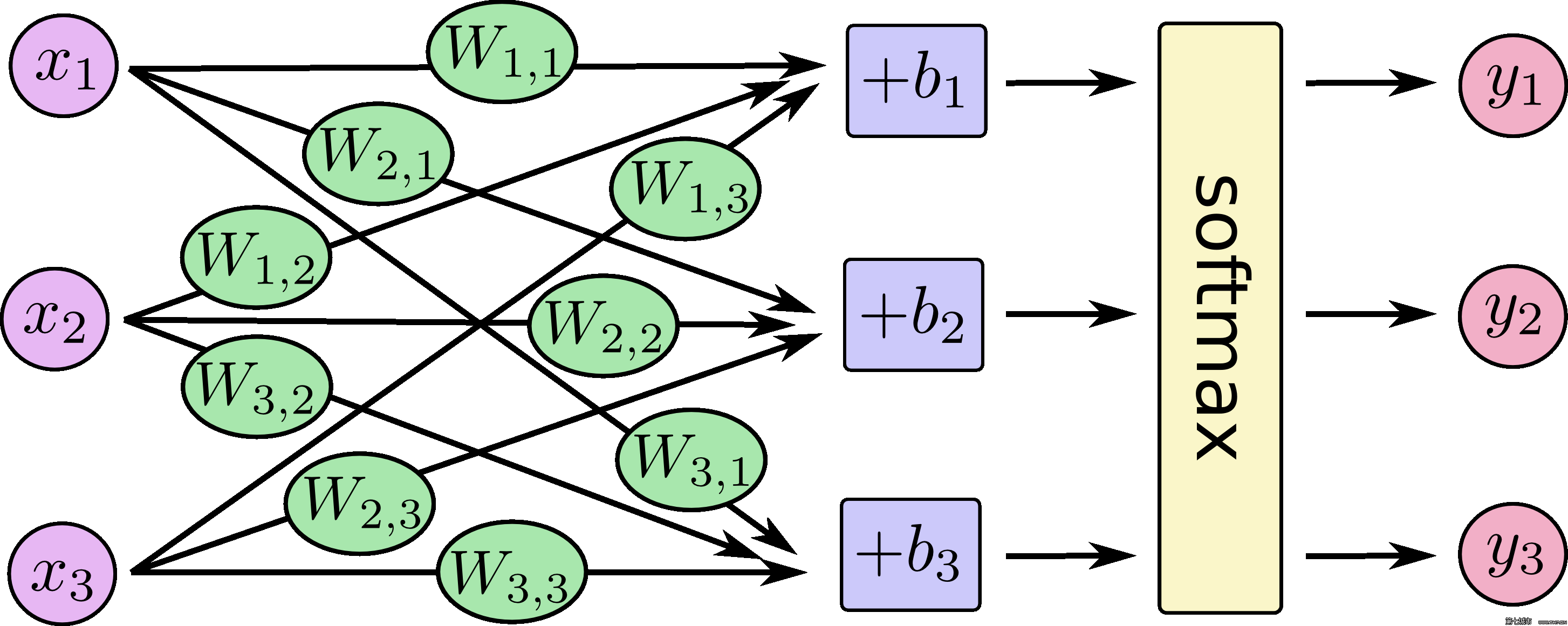
如果把它写成一个等式，我们可以得到：

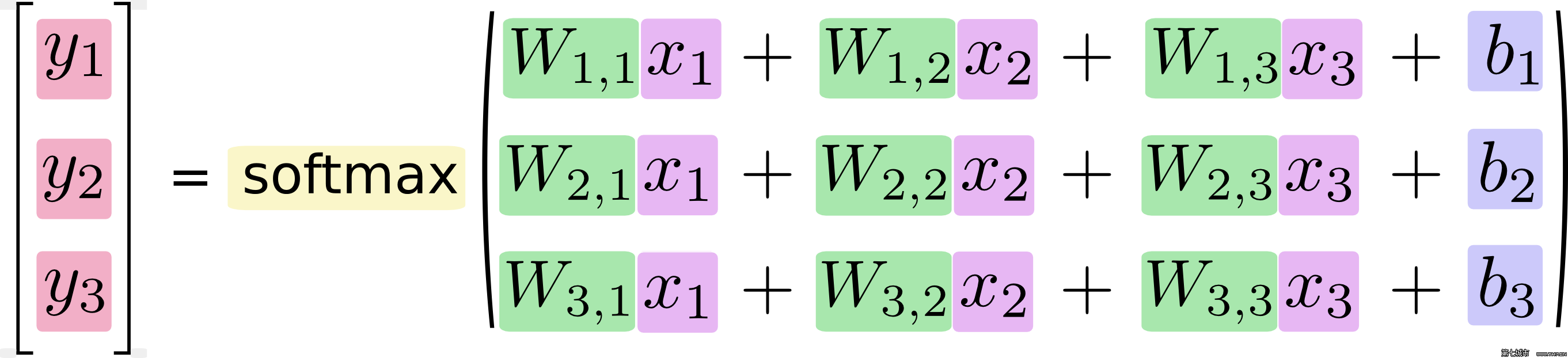
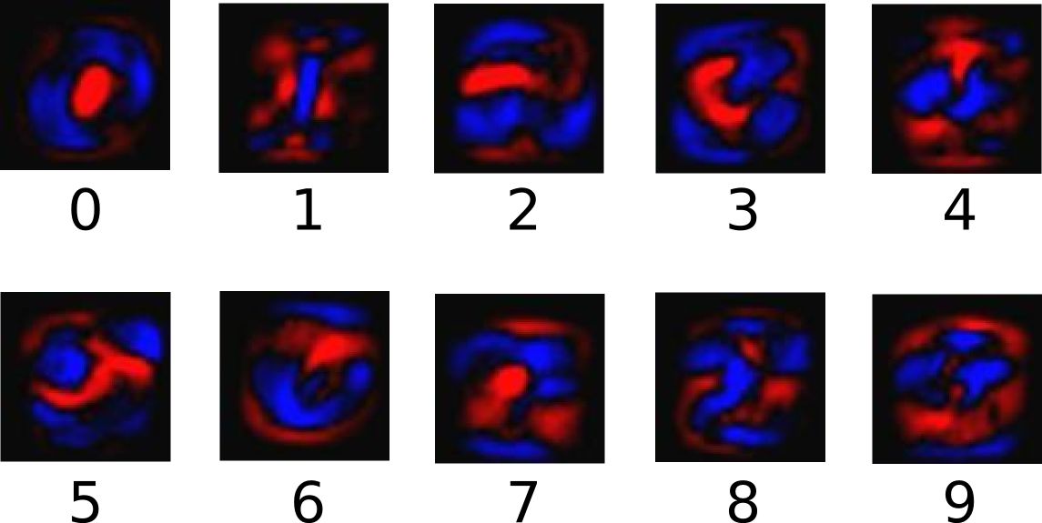
下面的图片显示了一个模型学习到的图片上每个像素对于特定数字类的权值。红色代表负数权值，蓝色代表正数权值。
（Hidden 层的所有权重 W 可排列成一个举证，则第 0 行的参数与数字为 0 的图运算后的概率会大于其他数字，想象成第 0 行的参数代表了 数字为 0 的图片）

Skip-gram 模型

三篇不错的译文
一文详解 Word2vec 之 Skip-Gram 模型（结构篇）
一文详解 Word2vec 之 Skip-Gram 模型（训练篇）
一文详解 Word2vec 之 Skip-Gram 模型（实现篇）

对于用词嵌入表示的文本向量，把一个词向量想象成一个图片，可得到相同的效果，只不过是向量的维度变大了

我们如何来表示这些单词呢？首先，我们都知道神经网络只能接受数值输入，我们不可能把一个单词字符串作为输入，因此我们得想个办法来表示这些单词。最常用的办法就是基于训练文档来构建我们自己的词汇表（vocabulary）再对单词进行one-hot编码

请参考：一文详解 Word2vec 之 Skip-Gram 模型（结构篇）

Word2Vec模型中，主要有Skip-Gram和CBOW两种模型，从直观上理解，Skip-Gram是给定input word来预测上下文。而CBOW是给定上下文，来预测input word

假如我们有一个句子“The dog barked at the mailman”，例如我们选取“dog”作为input word；

我们再定义一个叫做 skip_window 的参数，它代表着我们从当前 input word 的一侧（左边或右边）选取词的数量，如果我们设置skip_window=2，那么我们最终获得窗口中的词（包括input word在内）就是[‘The’, ‘dog’，’barked’, ‘at’]，所以整个窗口大小span=2x2=4

另一个参数叫 num_skips，它代表着我们从整个窗口中选取多少个不同的词作为我们的 output word，当skip_window=2，num_skips=2时，我们将会得到两组 (input word, output word) 形式的训练数据，即 (‘dog’, ‘barked’)，(‘dog’, ‘the’)

注意：这里我是直接 copy 一文详解 Word2vec 之 Skip-Gram 模型（结构篇） 的，这里当 skip_window=2，num_skips=2时，我觉得将得到三组(input word, output word) 形式的训练数据，即 (‘dog’, ‘barked’)，(‘dog’, ‘the’)，(‘dog’，’at’)
我没看懂原文为什么少了 (‘dog’，’at’)

当我们将文本数据输入后，就会产生很多的 (input word, output word) 形式的数据，这些才是真正的训练数据，我们可以把 input word 类比成一张 mnist 图片，对应的标签是 output word

我们选定句子“The quick brown fox jumps over lazy dog”，设定我们的窗口大小为2（window_size=2），也就是说我们仅选输入词前后各两个词和输入词进行组合。下图中，蓝色代表input word，方框内代表位于窗口内的单词。

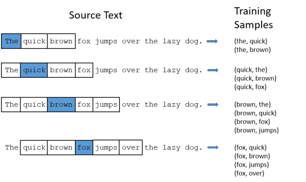
我们的模型将会从每对单词出现的次数中习得统计结果。例如，我们的神经网络可能会得到更多类似（“Soviet“，”Union“）这样的训练样本对，而对于（”Soviet“，”Sasquatch“）这样的组合却看到的很少。因此，当我们的模型完成训练后，给定一个单词”Soviet“作为输入，输出的结果中”Union“或者”Russia“要比”Sasquatch“被赋予更高的概率。

模型的输入如果为一个10000维的向量，那么输出也是一个10000维度（词汇表的大小）的向量，它包含了10000个概率，每一个概率代表着当前词是输入样本中output word的概率大小。

说完单词的编码和训练样本的选取，我们来看下我们的隐层。如果我们现在想用300个特征来表示一个单词（即每个词可以被表示为300维的向量）。那么隐层的权重矩阵应该为10000行，300列（隐层有300个结点）

看下面的图片，左右两张图分别从不同角度代表了输入层-隐层的权重矩阵。左图中每一列代表一个10000维的词向量和隐层单个神经元连接的权重向量。从右边的图来看，每一行实际上代表了每个单词的词向量

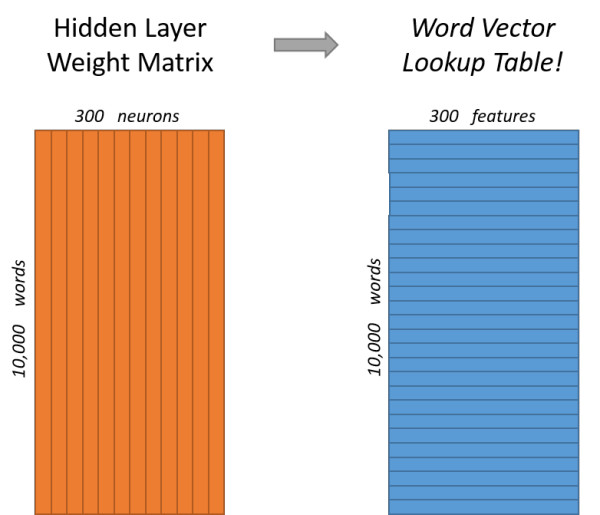
所以我们最终的目标就是学习这个隐层的权重矩阵。

我们现在回来接着通过模型的定义来训练我们的这个模型。

上面我们提到，input word和output word都会被我们进行one-hot编码。仔细想一下，我们的输入被one-hot编码以后大多数维度上都是0（实际上仅有一个位置为1），所以这个向量相当稀疏，那么会造成什么结果呢。如果我们将一个1 x 10000的向量和10000 x 300的矩阵相乘，它会消耗相当大的计算资源，为了高效计算，它仅仅会选择矩阵中对应的向量中维度值为1的索引行（这句话很绕），看图就明白

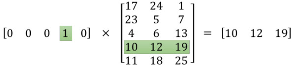
为了有效地进行计算，这种稀疏状态下不会进行矩阵乘法计算，可以看到矩阵的计算的结果实际上是矩阵对应的向量中值为1的索引，上面的例子中，左边向量中取值为1的对应维度为3（下标从0开始），那么计算结果就是矩阵的第3行（下标从0开始）—— [10, 12, 19]，这样模型中的隐层权重矩阵便成了一个”查找表“（lookup table），进行矩阵计算时，直接去查输入向量中取值为1的维度下对应的那些权重值。隐层的输出就是每个输入单词的“嵌入词向量”

TensorLayer的 word2vec 程序

""" 原文档：https://github.com/shorxp/tensorlayer-chinese/blob/master/example/tutorial_word2vec_basic.py Vector Representations of Words --------------------------------- This is the minimalistic reimplementation of tensorflow/examples/tutorials/word2vec/word2vec_basic.py This basic example contains the code needed to download some data, train on it a bit and visualize the result by using t-SNE. """
import collections
import math
import os
import random
import numpy as np
from six.moves import xrange  # pylint: disable=redefined-builtin
import tensorflow as tf
import tensorlayer as tl
import time
flags = tf.flags
flags.DEFINE_string("model", "one", "A type of model.")
FLAGS = flags.FLAGS
def main_word2vec_basic():
    """ Step 1: Download the data, read the context into a list of strings. Set hyperparameters. """
    words = tl.files.load_matt_mahoney_text8_dataset()
    word_list : a list
    # 单词列表
    # 例如： [.... 'the', 'cat', 'is', 'cute', ...]
    data_size = len(words)
    print('Data size', data_size) 
    resume = False  # 是否加载现有的模型、数据和字典
    _UNK = "_UNK"
    if FLAGS.model == "one":
        # toy setting 
        vocabulary_size = 50000 # 字典的长度
        batch_size = 128
        embedding_size = 128  # 词向量的维度
        skip_window = 1       # How many words to consider left and right.
        num_skips = 2         # How many times to reuse an input to generate a label.
                              # (should be double of 'skip_window' so as to
                              # use both left and right words)
        num_sampled = 64      # Number of negative examples to sample.
                              # more negative samples, higher loss
        learning_rate = 1.0
        n_epoch = 20          # 对整一个数据集循环训练的次数
        model_file_name = "model_word2vec_50k_128"
        # Eval 2084/15851 accuracy = 15.7%
    if FLAGS.model == "two":
        # (tensorflow/models/embedding/word2vec.py)
        vocabulary_size = 80000
        batch_size = 20     # Note: small batch_size need more steps for a Epoch
        embedding_size = 200
        skip_window = 5
        num_skips = 10
        num_sampled = 100
        learning_rate = 0.2
        n_epoch = 15
        model_file_name = "model_word2vec_80k_200"
        # 7.9%
    if FLAGS.model == "three":
        # (tensorflow/models/embedding/word2vec_optimized.py)
        vocabulary_size = 80000
        batch_size = 500
        embedding_size = 200
        skip_window = 5
        num_skips = 10
        num_sampled = 25
        learning_rate = 0.025
        n_epoch = 20
        model_file_name = "model_word2vec_80k_200_opt"
        # bad 0%
    if FLAGS.model == "four":
        # see: Learning word embeddings efficiently with noise-contrastive estimation
        vocabulary_size = 80000
        batch_size = 100
        embedding_size = 600
        skip_window = 5
        num_skips = 10
        num_sampled = 25
        learning_rate = 0.03
        n_epoch = 200 * 10
        model_file_name = "model_word2vec_80k_600"
        # bad
    # num_steps 整个一个训练过程中训练的批次，每批训练 batch_size 个数据
    num_steps = int((data_size/batch_size) * n_epoch)   # total number of iteration，一个 iteration 即一批，调用一次 tl.nlp.generate_skip_gram_batch
    print('%d Steps a Epoch, total Epochs %d' % (int(data_size/batch_size), n_epoch))
    print(' learning_rate: %f' % learning_rate)
    print(' batch_size: %d' % batch_size)
    """ Step 2: 建立词典，并用 'UNK' 代替不常见的词 """
    print()
    if resume:
        # 加载已经训练好的模型，数据和字典
        print("Load existing data and dictionaries" + "!"*10)
        all_var = tl.files.load_npy_to_any(name=model_file_name+'.npy')
        data = all_var['data']; count = all_var['count']
        dictionary = all_var['dictionary']
        reverse_dictionary = all_var['reverse_dictionary']
    else:
        data, count, dictionary, reverse_dictionary = \
                tl.nlp.build_words_dataset(words, vocabulary_size, True, _UNK)
    print('Most 5 common words (+UNK)', count[:5]) 
    # 词频最高的5个词： [['UNK', 418391], (b'the', 1061396), (b'of', 593677), (b'and', 416629), (b'one', 411764)]
    print('Sample data', data[:10], [reverse_dictionary[i] for i in data[:10]]) 
    # 输出前前10个数据，data中是词对应的id，reverse_dictionary中是词
    # [5243, 3081, 12, 6, 195, 2, 3135, 46, 59, 156] 
    # [b'anarchism', b'originated', b'as', b'a', b'term', b'of', b'abuse', b'first', b'used', b'against']
    del words  # 删除词列表 words 以减少内存占用
    """ Step 3: Function to generate a training batch for the Skip-Gram model. """
    print()
    data_index = 0
    batch, labels, data_index = tl.nlp.generate_skip_gram_batch(data=data,
                        batch_size=20, num_skips=4, skip_window=2, data_index=0)
    for i in range(20):
        print(batch[i], reverse_dictionary[batch[i]],
            '->', labels[i, 0], reverse_dictionary[labels[i, 0]])
    """ Step 4: Build a Skip-Gram model. """
    print()
    valid_size = 16     # 随机获取一些词来验证相似性
    valid_window = 100  # Only pick dev samples in the head of the distribution.
    valid_examples = np.random.choice(valid_window, valid_size, replace=False)
    # print(valid_examples) # [90 85 20 33 35 62 37 63 88 38 82 58 83 59 48 64]
    print_freq = 2000
    # n_epoch = int(num_steps / batch_size) 训练数据集的轮数
    # train_inputs 是一个向量, 每个不同的词对应一个id
    # train_labels is a column vector, 即一个词所对应的向量
    # valid_dataset is a column vector, a valid set is an integer id of single word.
    train_inputs = tf.placeholder(tf.int32, shape=[batch_size])
    train_labels = tf.placeholder(tf.int32, shape=[batch_size, 1])
    valid_dataset = tf.constant(valid_examples, dtype=tf.int32)
    # Look up embeddings for inputs.
    emb_net = tl.layers.Word2vecEmbeddingInputlayer(
            inputs = train_inputs,
            train_labels = train_labels,
            vocabulary_size = vocabulary_size,
            embedding_size = embedding_size,
            num_sampled = num_sampled,
            nce_loss_args = {},
            E_init = tf.random_uniform_initializer(minval=-1.0, maxval=1.0),
            E_init_args = {},
            nce_W_init = tf.truncated_normal_initializer(stddev=float(1.0/np.sqrt(embedding_size))),
            nce_W_init_args = {},
            nce_b_init = tf.constant_initializer(value=0.0),
            nce_b_init_args = {},
            name ='word2vec_layer',
        )
    # 优化函数
    cost = emb_net.nce_cost
    train_params = emb_net.all_params
    # train_op = tf.train.GradientDescentOptimizer(learning_rate).minimize(cost, var_list=train_params)
    train_op = tf.train.AdagradOptimizer(learning_rate, initial_accumulator_value=0.1,
        use_locking=False).minimize(cost, var_list=train_params)
    # Compute the cosine similarity between minibatch examples and all embeddings.
    # For simple visualization of validation set.
    normalized_embeddings = emb_net.normalized_embeddings
    # tf.nn.embedding_lookup 对批数据中的单词建立嵌套向量
    valid_embed = tf.nn.embedding_lookup(
                                normalized_embeddings, valid_dataset)
    similarity = tf.matmul(
        valid_embed, normalized_embeddings, transpose_b=True)
        # multiply all valid word vector with all word vector.
        # transpose_b=True, normalized_embeddings is transposed before multiplication.
    """ Step 5: Begin training. """
    print()
    sess.run(tf.initialize_all_variables())
    if resume:
        print("Load existing model" + "!"*10)
        # Load from ckpt or npz file
        saver = tf.train.Saver()
        saver.restore(sess, model_file_name+'.ckpt')
        # load_params = tl.files.load_npz(name=model_file_name+'.npz')
        # tl.files.assign_params(sess, load_params, emb_net)
    emb_net.print_params()
    emb_net.print_layers()
    # save vocabulary to txt
    tl.nlp.save_vocab(count, name='vocab_text8.txt')
    average_loss = 0
    # for step in xrange(num_steps):
    step = 0
    while (step < num_steps):
        start_time = time.time()
        batch_inputs, batch_labels, data_index = tl.nlp.generate_skip_gram_batch(
                        data=data, batch_size=batch_size, num_skips=num_skips,
                        skip_window=skip_window, data_index=data_index)
        feed_dict = {train_inputs : batch_inputs, train_labels : batch_labels}
        # We perform one update step by evaluating the train_op (including it
        # in the list of returned values for sess.run()
        _, loss_val = sess.run([train_op, cost], feed_dict=feed_dict)
        average_loss += loss_val
        if step % print_freq == 0:
            if step > 0:
                average_loss /= 2000
            print("Average loss at step %d/%d. loss:%f took:%fs" %
                        (step, num_steps, average_loss, time.time() - start_time))
            average_loss = 0
        # Prints out nearby words given a list of words.
        # Note that this is expensive (~20% slowdown if computed every 500 steps)
        if step % (print_freq * 5) == 0:
            sim = similarity.eval()
            for i in xrange(valid_size):
                valid_word = reverse_dictionary[valid_examples[i]]
                top_k = 8 # number of nearest neighbors to print
                nearest = (-sim[i, :]).argsort()[1:top_k+1]
                log_str = "Nearest to %s:" % valid_word
                for k in xrange(top_k):
                    close_word = reverse_dictionary[nearest[k]]
                    log_str = "%s %s," % (log_str, close_word)
                print(log_str)
        if (step % (print_freq * 20) == 0) and (step != 0):
            print("Save model, data and dictionaries" + "!"*10);
            # Save to ckpt or npz file
            saver = tf.train.Saver()
            save_path = saver.save(sess,"./" + model_file_name +'.ckpt')
            # tl.files.save_npz(emb_net.all_params, name=model_file_name+'.npz')
            tl.files.save_any_to_npy(save_dict={
   'data': data, 'count': count,
                'dictionary': dictionary, 'reverse_dictionary':
                reverse_dictionary}, name=model_file_name+'.npy')
        if step == num_steps-1:
            keeptrain = input("Training %d finished enter 1 to keep training: " % num_steps)
            if keeptrain == '1':
                step = 0
                learning_rate = float(input("Input new learning rate: "))
                train_op = tf.train.GradientDescentOptimizer(learning_rate).minimize(cost)
        step += 1
    """ Step 6: Visualize the normalized embedding matrix by t-SNE. """
    print()
    final_embeddings = normalized_embeddings.eval()
    tl.visualize.tsne_embedding(final_embeddings, reverse_dictionary,
                plot_only=500, second=5, saveable=False, name='word2vec_basic')
    """ Step 7: Evaluate by analogy questions. see tensorflow/models/embedding/word2vec_optimized.py """
    print()
    # from tensorflow/models/embedding/word2vec.py
    analogy_questions = tl.nlp.read_analogies_file( \
                eval_file='questions-words.txt', word2id=dictionary)
    # The eval feeds three vectors of word ids for a, b, c, each of
    # which is of size N, where N is the number of analogies we want to
    # evaluate in one batch.
    analogy_a = tf.placeholder(dtype=tf.int32)  # [N]
    analogy_b = tf.placeholder(dtype=tf.int32)  # [N]
    analogy_c = tf.placeholder(dtype=tf.int32)  # [N]
    # Each row of a_emb, b_emb, c_emb is a word's embedding vector.
    # They all have the shape [N, emb_dim]
    a_emb = tf.gather(normalized_embeddings, analogy_a)  # a's embs
    b_emb = tf.gather(normalized_embeddings, analogy_b)  # b's embs
    c_emb = tf.gather(normalized_embeddings, analogy_c)  # c's embs
    # We expect that d's embedding vectors on the unit hyper-sphere is
    # near: c_emb + (b_emb - a_emb), which has the shape [N, emb_dim].
    # Bangkok Thailand Tokyo Japan -> Thailand - Bangkok = Japan - Tokyo
    # Japan = Tokyo + (Thailand - Bangkok)
    # d = c + (b - a)
    target = c_emb + (b_emb - a_emb)
    # Compute cosine distance between each pair of target and vocab.
    # dist has shape [N, vocab_size].
    dist = tf.matmul(target, normalized_embeddings, transpose_b=True)
    # For each question (row in dist), find the top 'n_answer' words.
    n_answer = 4
    _, pred_idx = tf.nn.top_k(dist, n_answer)
    def predict(analogy):
        """Predict the top 4 answers for analogy questions."""
        idx, = sess.run([pred_idx], {
            analogy_a: analogy[:, 0],
            analogy_b: analogy[:, 1],
            analogy_c: analogy[:, 2]
        })
        return idx
    # Evaluate analogy questions and reports accuracy.
    # i.e. How many questions we get right at precision@1.
    correct = 0
    total = analogy_questions.shape[0]
    start = 0
    while start < total:
        limit = start + 2500
        sub = analogy_questions[start:limit, :] # question
        idx = predict(sub)      # 4 answers for each question
        # print('question:', tl.nlp.word_ids_to_words(sub[0], reverse_dictionary))
        # print('answers:', tl.nlp.word_ids_to_words(idx[0], reverse_dictionary))
        start = limit
        for question in xrange(sub.shape[0]):
            for j in xrange(n_answer):
                # if one of the top 4 answers in correct, win !
                if idx[question, j] == sub[question, 3]:
                    # Bingo! We predicted correctly. E.g., [italy, rome, france, paris].
                    print(j+1, tl.nlp.word_ids_to_words([idx[question, j]], reverse_dictionary) \
                        , ':', tl.nlp.word_ids_to_words(sub[question, :], reverse_dictionary))
                    correct += 1
                    break
                elif idx[question, j] in sub[question, :3]:
                    # We need to skip words already in the question.
                    continue
                else:
                    # The correct label is not the precision@1
                    break
    print("Eval %4d/%d accuracy = %4.1f%%" % (correct, total,
                                             correct * 100.0 / total))
if __name__ == '__main__':
    sess = tf.InteractiveSession()
    main_word2vec_basic()

输出结果

Nearest to by: through, including, in, under, during, via, from, featuring,
Nearest to years: decades, weeks, days, months, hours, seconds, minutes, year,
Nearest to used: employed, needed, referred, presented, designed, cited, applied, adopted,
Nearest to has: had, have, is, was, maintains, requires, produces, since,
Nearest to of: including, in, besides, from, for, although, includes, and,
Nearest to see: references, but, compare, include, etc, and, external, refers,
Nearest to war: wars, conflict, atrocities, veterans, turmoil, crisis, battle, wwii,
Nearest to that: which, however, nevertheless, additionally, what, moreover, but, furthermore,
Nearest to th: nd, ninth, rd, seventh, twentieth, tenth, nineteenth, st,
Nearest to states: kingdom, nations, state, countries, us, organizations, nation, netherlands,
Nearest to about: approximately, over, regarding, concerning, around, exactly, roughly, within,
Nearest to five: four, seven, six, three, eight, two, nine, zero,
Nearest to his: her, their, my, its, your, our, the, whose,
Nearest to zero: five, seven, eight, six, four, nine, three, two,
Nearest to system: systems, scheme, model, mechanisms, mechanism, theory, concept, process,
Nearest to be: been, become, get, have, is, seem, refer, prove,
Average loss at step 2652000/2657063. loss:3.958110 took:0.002000s
Average loss at step 2654000/2657063. loss:3.956920 took:0.002000s
Average loss at step 2656000/2657063. loss:3.973455 took:0.002000s

参考文档：

1. TensorFlow 字词的向量表示 http://www.tensorfly.cn/tfdoc/tutorials/word2vec.html
2. Wikipedia Vector space model https://en.wikipedia.org/wiki/Vector_space_model
3. 维基百科 自然语言处理
   https://zh.wikipedia.org/wiki/%E8%87%AA%E7%84%B6%E8%AF%AD%E8%A8%80%E5%A4%84%E7%90%86