Does sentiment analysis work? A tidy analysis of Yelp reviews
This year Julia Silge and I released the tidytext package for text mining using tidy tools such as dplyr, tidyr, ggplot2 and broom. One of the canonical examples of tidy text mining this package makes possible is sentiment analysis.
Sentiment analysis is often used by companies to quantify general social media opinion (for example, using tweets about several brands to compare customer satisfaction). One of the simplest and most common sentiment analysis methods is to classify words as “positive” or “negative”, then to average the values of each word to categorize the entire document. (See this vignette andJulia’s post for examples of a tidy application of sentiment analysis). But does this method actually work? Can you predict the positivity or negativity of someone’s writing by counting words?
To answer this, let’s try sentiment analysis on a text dataset where we know the “right answer”- one where each customer also quantified their opinion. In particular, we’ll use the Yelp Dataset: a wonderful collection of millions of restaurant reviews, each accompanied by a 1-5 star rating. We’ll try out a specific sentiment analysis method, and see the extent to which we can predict a customer’s rating based on their written opinion. In the process we’ll get a sense of the strengths and weaknesses of sentiment analysis, and explore another example of tidy text mining with tidytext, dplyr, and ggplot2.
Setup
I’ve downloaded theyelp_dataset_challenge_academic_dataset folder from here.1First I read and process them into a data frame:
library(stringr) library(jsonlite) # Each line is a JSON object- the fastest way to process is to combine into a # single JSON string and use fromJSON and flatten reviews_combined <- str_c("[", str_c(review_lines, collapse = ", "), "]") reviews <- fromJSON(reviews_combined) %>% flatten() %>% tbl_df()
We now have a data frame with one row per review:
reviews## # A tibble: 200,000 x 10## user_id review_id stars date## <chr> <chr> <int> <chr>## 1 PUFPaY9KxDAcGqfsorJp3Q Ya85v4eqdd6k9Od8HbQjyA 4 2012-08-01## 2 Iu6AxdBYGR4A0wspR9BYHA KPvLNJ21_4wbYNctrOwWdQ 5 2014-02-13## 3 auESFwWvW42h6alXgFxAXQ fFSoGV46Yxuwbr3fHNuZig 5 2015-10-31## 4 uK8tzraOp4M5u3uYrqIBXg Di3exaUCFNw1V4kSNW5pgA 5 2013-11-08## 5 I_47G-R2_egp7ME5u_ltew 0Lua2-PbqEQMjD9r89-asw 3 2014-03-29## 6 PP_xoMSYlGr2pb67BbqBdA 7N9j5YbBHBW6qguE5DAeyA 1 2014-10-29## 7 JPPhyFE-UE453zA6K0TVgw mjCJR33jvUNt41iJCxDU_g 4 2014-11-28## 8 2d5HeDvZTDUNVog_WuUpSg Ieh3kfZ-5J9pLju4JiQDvQ 5 2014-02-27## 9 BShxMIUwaJS378xcrz4Nmg PU28OoBSHpZLkYGCmNxlmg 5 2015-06-16## 10 fhNxoMwwTipzjO8A9LFe8Q XsA6AojkWjOHA4FmuAb8XQ 3 2012-08-19## # ... with 199,990 more rows, and 6 more variables: text <chr>,## # type <chr>, business_id <chr>, votes.funny <int>, votes.useful <int>,## # votes.cool <int>
Notice the stars column with the star rating the user gave, as well as the text column (too large to display) with the actual text of the review. For now, we’ll focus on whether we can predict the star rating based on the text.
Tidy sentiment analysis
Right now, there is one row for each review. To analyze in the tidy text framework, we need to use the unnest_tokens function and turn this into one-row-per-term-per-document:
library(tidytext) review_words <- reviews %>% select(review_id, business_id, stars, text) %>% unnest_tokens(word, text) %>% filter(!word %in% stop_words$word, str_detect(word, "^[a-z']+$")) review_words## # A tibble: 7,688,667 x 4## review_id business_id stars word## <chr> <chr> <int> <chr>## 1 Ya85v4eqdd6k9Od8HbQjyA 5UmKMjUEUNdYWqANhGckJw 4 hoagie## 2 Ya85v4eqdd6k9Od8HbQjyA 5UmKMjUEUNdYWqANhGckJw 4 institution## 3 Ya85v4eqdd6k9Od8HbQjyA 5UmKMjUEUNdYWqANhGckJw 4 walking## 4 Ya85v4eqdd6k9Od8HbQjyA 5UmKMjUEUNdYWqANhGckJw 4 throwback## 5 Ya85v4eqdd6k9Od8HbQjyA 5UmKMjUEUNdYWqANhGckJw 4 ago## 6 Ya85v4eqdd6k9Od8HbQjyA 5UmKMjUEUNdYWqANhGckJw 4 fashioned## 7 Ya85v4eqdd6k9Od8HbQjyA 5UmKMjUEUNdYWqANhGckJw 4 menu## 8 Ya85v4eqdd6k9Od8HbQjyA 5UmKMjUEUNdYWqANhGckJw 4 board## 9 Ya85v4eqdd6k9Od8HbQjyA 5UmKMjUEUNdYWqANhGckJw 4 booths## 10 Ya85v4eqdd6k9Od8HbQjyA 5UmKMjUEUNdYWqANhGckJw 4 selection## # ... with 7,688,657 more rows
Notice that there is now one-row-per-term-per-document: the tidy text form. In this cleaning process we’ve also removed “stopwords” (such as “I”, “the”, “and”, etc), and removing things things that are formatting (e.g. “—-“) rather than a word.
Now let’s perform sentiment analysis on each review. We’ll use the AFINN lexicon, which provides a positivity score for each word, from -5 (most negative) to 5 (most positive). This, along with several other lexicons, are stored in the sentiments table that comes with tidytext. (I’ve tried some other lexicons on this dataset and the results are pretty similar.)
AFINN <- sentiments %>% filter(lexicon == "AFINN") %>% select(word, afinn_score = score) AFINN## # A tibble: 2,476 x 2## word afinn_score## <chr> <int>## 1 abandon -2## 2 abandoned -2## 3 abandons -2## 4 abducted -2## 5 abduction -2## 6 abductions -2## 7 abhor -3## 8 abhorred -3## 9 abhorrent -3## 10 abhors -3## # ... with 2,466 more rows
Now as described in Julia’s post, our sentiment analysis is just an inner-join operation followed by a summary:
reviews_sentiment <- review_words %>% inner_join(AFINN, by = "word") %>% group_by(review_id, stars) %>% summarize(sentiment = mean(afinn_score)) reviews_sentiment## Source: local data frame [187,688 x 3]## Groups: review_id [?]#### review_id stars sentiment## (chr) (int) (dbl)## 1 __-r0eC3hZlaejvuliC8zQ 5 4.0000000## 2 __1yzxN39QzdeJqicAg99A 3 1.3333333## 3 __3Vy9VLHV5jKjgFDRWCiQ 2 1.3333333## 4 __56FUEaW57kZEm56OZk7w 5 0.8333333## 5 __5webDfFxADKz_3k5YipA 5 2.2222222## 6 __6QkPtePef4_oW6A_tbOg 4 2.0000000## 7 __6tOxx2VcvGR02d2ILkuw 5 1.7500000## 8 __77nP3Nf1wsGz5HPs2hdw 5 1.6000000## 9 __7MkcofSZYHj9v5KuLVvQ 4 1.8333333## 10 __7RBFUZgxef8gZ8guaVhg 5 2.4000000## .. ... ... ...
We now have an average sentiment alongside the star ratings. If we’re right and sentiment analysis can predict a review’s opinion towards a restaurant, we should expect the sentiment score to correlate with the star rating.
Did it work?
library(ggplot2) theme_set(theme_bw())ggplot(reviews_sentiment, aes(stars, sentiment, group = stars)) + geom_boxplot() + ylab("Average sentiment score")
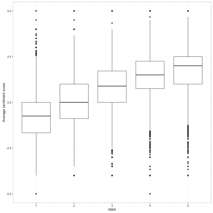
Well, it’s a very good start! Our sentiment scores are certainly correlated with positivity ratings. But we do see that there’s a large amount of prediction error- some 5-star reviews have a highly negative sentiment score, and vice versa.
Which words are positive or negative?
Our algorithm works at the word level, so if we want to improve our approach we should start there. Which words are suggestive of positive reviews, and which are negative?
To examine this, let’s create a per-word summary, and see which words tend to appear in positive or negative reviews. This takes more grouping and summarizing:
review_words_counted <- review_words %>% count(review_id, business_id, stars, word) %>% ungroup() review_words_counted## # A tibble: 6,566,367 x 5## review_id business_id stars word n## <chr> <chr> <int> <chr> <int>## 1 ___XYEos-RIkPsQwplRYyw YxMnfznT3eYya0YV37tE8w 5 batter 1## 2 ___XYEos-RIkPsQwplRYyw YxMnfznT3eYya0YV37tE8w 5 chips 3## 3 ___XYEos-RIkPsQwplRYyw YxMnfznT3eYya0YV37tE8w 5 compares 1## 4 ___XYEos-RIkPsQwplRYyw YxMnfznT3eYya0YV37tE8w 5 fashioned 1## 5 ___XYEos-RIkPsQwplRYyw YxMnfznT3eYya0YV37tE8w 5 filleted 1## 6 ___XYEos-RIkPsQwplRYyw YxMnfznT3eYya0YV37tE8w 5 fish 4## 7 ___XYEos-RIkPsQwplRYyw YxMnfznT3eYya0YV37tE8w 5 fries 1## 8 ___XYEos-RIkPsQwplRYyw YxMnfznT3eYya0YV37tE8w 5 frozen 1## 9 ___XYEos-RIkPsQwplRYyw YxMnfznT3eYya0YV37tE8w 5 greenlake 1## 10 ___XYEos-RIkPsQwplRYyw YxMnfznT3eYya0YV37tE8w 5 hand 1## # ... with 6,566,357 more rowsword_summaries <- review_words_counted %>% group_by(word) %>% summarize(businesses = n_distinct(business_id), reviews = n(), uses = sum(n), average_stars = mean(stars)) %>% ungroup() word_summaries## # A tibble: 100,177 x 5## word businesses reviews uses average_stars## <chr> <int> <int> <int> <dbl>## 1 a'boiling 1 1 1 4.0## 2 a'fare 1 1 1 4.0## 3 a'hole 1 1 1 5.0## 4 a'ight 6 6 6 2.5## 5 a'la 2 2 2 4.5## 6 a'll 1 1 1 1.0## 7 a'lyce 1 1 2 5.0## 8 a'more 1 2 2 5.0## 9 a'orange 1 1 1 5.0## 10 a'prowling 1 1 1 3.0## # ... with 100,167 more rows
We can start by looking only at words that appear in at least 200 (out of 200000) reviews. This makes sense both because rare words will have a noisier measurement (a few good or bad reviews could shift the balance), and because they’re less likely to be useful in classifying future reviews or text. I also filter for ones that appear in at least 10 businesses (others are likely to be specific to a particular restaurant).
word_summaries_filtered <- word_summaries %>% filter(reviews >= 200, businesses >= 10) word_summaries_filtered## # A tibble: 4,328 x 5## word businesses reviews uses average_stars## <chr> <int> <int> <int> <dbl>## 1 ability 374 402 410 3.465174## 2 absolute 808 1150 1183 3.710435## 3 absolutely 2728 6158 6538 3.757389## 4 ac 378 646 919 3.191950## 5 accent 171 203 214 3.285714## 6 accept 557 720 772 2.929167## 7 acceptable 500 587 608 2.505963## 8 accepted 293 321 332 2.968847## 9 access 544 840 925 3.505952## 10 accessible 220 272 282 3.816176## # ... with 4,318 more rows
What were the most positive and negative words?
word_summaries_filtered %>% arrange(desc(average_stars))## # A tibble: 4,328 x 5## word businesses reviews uses average_stars## <chr> <int> <int> <int> <dbl>## 1 compassionate 193 298 312 4.677852## 2 listens 177 215 218 4.632558## 3 exceeded 286 320 321 4.596875## 4 painless 224 290 294 4.568966## 5 knowledgable 607 775 786 4.549677## 6 gem 874 1703 1733 4.537874## 7 impeccable 278 475 477 4.520000## 8 happier 545 638 654 4.495298## 9 knowledgeable 1550 2747 2807 4.493629## 10 compliments 333 418 428 4.488038## # ... with 4,318 more rows
Looks plausible to me! What about negative?
word_summaries_filtered %>% arrange(average_stars)## # A tibble: 4,328 x 5## word businesses reviews uses average_stars## <chr> <int> <int> <int> <dbl>## 1 scam 211 263 297 1.368821## 2 incompetent 275 317 337 1.378549## 3 unprofessional 748 921 988 1.380022## 4 disgusted 251 283 292 1.381625## 5 rudely 349 391 418 1.493606## 6 lied 281 332 372 1.496988## 7 refund 717 930 1229 1.545161## 8 unacceptable 387 441 449 1.569161## 9 worst 2574 5107 5597 1.569219## 10 refused 803 983 1096 1.579858## # ... with 4,318 more rows
Also makes a lot of sense. We can also plot positivity by frequency:
ggplot(word_summaries_filtered, aes(reviews, average_stars)) + geom_point() + geom_text(aes(label = word), check_overlap = TRUE, vjust = 1, hjust = 1) + scale_x_log10() + geom_hline(yintercept = mean(reviews$stars), color = "red", lty = 2) + xlab("# of reviews") + ylab("Average Stars")
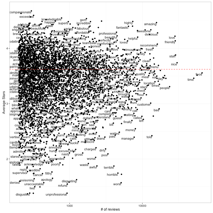
Note that some of the most common words (e.g. “food”) are pretty neutral. There are some common words that are pretty positive (e.g. “amazing”, “awesome”) and others that are pretty negative (“bad”, “told”).
Comparing to sentiment analysis
When we perform sentiment analysis, we’re typically comparing to a pre-existing lexicon, one that may have been developed for a particular purpose. That means that on our new dataset (Yelp reviews), some words may have different implications.
We can combine and compare the two datasets with inner_join.
words_afinn <- word_summaries_filtered %>% inner_join(AFINN) words_afinn## # A tibble: 505 x 6## word businesses reviews uses average_stars afinn_score## <chr> <int> <int> <int> <dbl> <int>## 1 ability 374 402 410 3.465174 2## 2 accept 557 720 772 2.929167 1## 3 accepted 293 321 332 2.968847 1## 4 accident 369 447 501 3.536913 -2## 5 accidentally 279 305 307 3.252459 -2## 6 active 177 215 238 3.744186 1## 7 adequate 420 502 527 3.203187 1## 8 admit 942 1316 1348 3.620821 -1## 9 admitted 196 248 271 2.157258 -1## 10 adorable 305 416 431 4.281250 3## # ... with 495 more rowsggplot(words_afinn, aes(afinn_score, average_stars, group = afinn_score)) + geom_boxplot() + xlab("AFINN score of word") + ylab("Average stars of reviews with this word")

Just like in our per-review predictions, there’s a very clear trend. AFINN sentiment analysis works, at least a little bit!
But we may want to see some of those details. Which positive/negative words were most successful in predicting a positive/negative review, and which broke the trend?
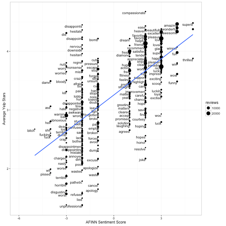
For example, we can see that most profanity has an AFINN score of -4, and that while some words, like “wtf”, successfully predict a negative review, others, like “damn”, are often positive (e.g. “the roast beef was damn good!”). Some of the words that AFINN most underestimated included “die” (“the pork chops are to diefor!”), and one of the words it most overestimated was “joke” (“the service is a complete joke!”).
One other way we could look at misclassifications is to add AFINN sentiments to our frequency vs average stars plot:
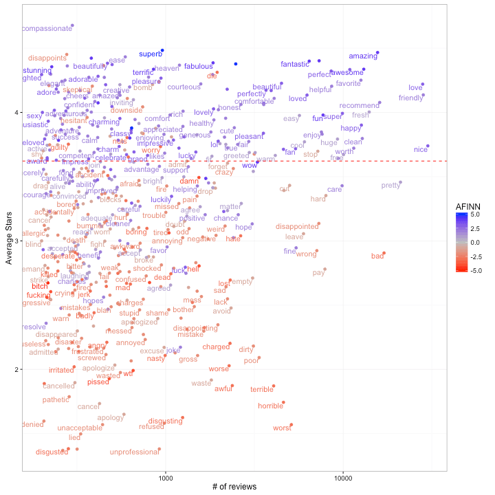
One thing I like about the tidy text mining framework is that it lets us explore the successes and failures of our model at this granular level, using tools (ggplot2, dplyr) that we’re already familiar with.
Next time: Machine learning
In this post I’ve focused on basic exploration of the Yelp review dataset, and an evaluation of one sentiment analysis method for predicting review positivity. (Our conclusion: it’s good, but far from perfect!) But what if we want to create our own prediction method based on these reviews?
In my next post on this topic, I’ll show how to train LASSO regression (with the glmnet package) on this dataset to create a predictive model. This will serve as an introduction to machine learning methods in text classification. It will also let us create our own new “lexicon” of positive and negative words, one that may be more appropriate to our context of restaurant reviews.
- I encourage you to download this dataset and follow along- but note that if you do, you are bound by their Terms of Use.


还没有评论,来说两句吧...