人工智能-深度学习-手写数字识别
1.准备数据
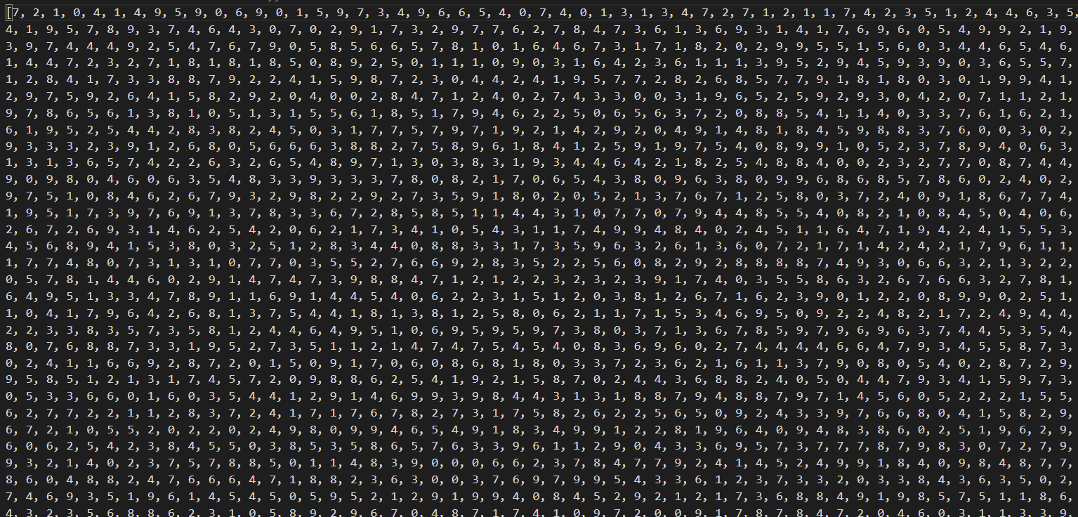
手写数字识别的特征集是一组数值为0-9,大小为 28 * 28 矩阵的图片, 标签为与之对应的数字:
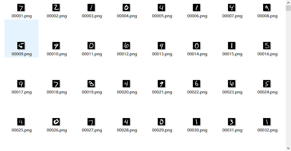
数据下载链接: 手写数字识别数据集
2.将数据格式化为 npz 文件
""" 将图片和标签整理为 npz 文件 """import numpy as npimport osfrom PIL import Imageimport json# 读取图片# 存到 npz 文件中的为 28 *28 的矩阵列表train_file_path = "nums/train_x/"train_x = []for root, dirs, files in os.walk(train_file_path):for f in files:img = np.array(Image.open(os.path.join(root, f)))train_x.append(img)test_file_path = "nums/test_x/"test_x = []for root, dirs, files in os.walk(test_file_path):for f in files:img = np.array(Image.open(os.path.join(root, f)))test_x.append(img)train_object = open('nums/train_y.json', 'r')train_y = json.load(train_object)test_object = open('nums/test_y.json', 'r')test_y = json.load(test_object)np.savez('nums.npz', train_x=np.array(train_x), test_x=np.array(test_x),train_y=np.array(train_y), test_y=np.array(test_y))
我们顺便记录下, 如何把npz里的数据还原成图片和json文件
""" 从 nums.npz 中读取各个图片和各自的标签 """import numpy as npfrom PIL import Imageimport json# 加载数据image_data = np.load("data/mnist.npz")# 分别获取训练集和数据集x_train = image_data["x_train"]y_train = image_data["y_train"]x_test = image_data["x_test"]y_test = image_data["y_test"]# 分别把训练集和测试集恢复为png 图片for i in range(len(x_train)):im = Image.fromarray(x_train[i])im.save("nums/train_x/%05d.png" % (i + 1))for i in range(len(x_test)):im = Image.fromarray(x_test[i])im.save("nums/test_x/%05d.png" % (i + 1))# 分别把训练集和测试集的标签写入到json文件中train_num_writer = open("nums/train_y.json", 'w')train_num_writer.write(json.dumps(y_train.tolist(), ensure_ascii=False))train_num_writer.close()test_num_writer = open("nums/test_y.json", 'w')test_num_writer.write(json.dumps(y_test.tolist(), ensure_ascii=False))test_num_writer.close()
3.训练
采用交叉熵作为损失函数, 28* 28 的784个像素值作为特征向量, 这种训练方式很暴力, 后期如果有其他更精巧的训练方式再来补充, 大家可以先把这种训练当成深度学习中的hello world
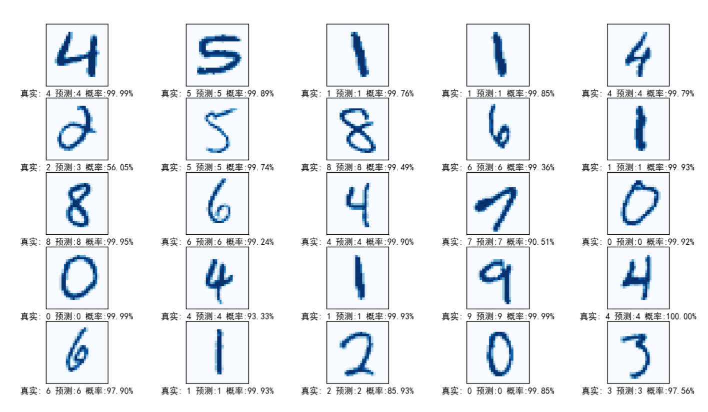
""" 手写数字识别(以交叉熵为激活函数的深度学习) """import torchimport torch.nn as nnimport torch.nn.functional as fcimport numpy as npimport matplotlib.pyplot as pltimport matplotlib.gridspec as grid_specplt.switch_backend("TkAgg")# 一. 准备训练集和测试集数据# 从npz文件中加载数据image_data = np.load("nums.npz")# 获取训练集数据, 并将每张图片的 28 * 28 的矩阵转变为 1 * 784 的矩阵, 转为浮点数# 除以 255 是为了# 即我们把 784 个像素点的值处理后当做 784 个特征, 测试集特征同样如此train_x = image_data["train_x"].reshape([-1, 784]).astype(np.float32) / 255# 获取标签, 每个标签为图片对应的数字train_y = image_data["train_y"].astype(np.float32)# 获取测试集数据test_x = image_data["test_x"].reshape([-1, 784]).astype(np.float32) / 255test_y = image_data["test_y"].astype(np.float32)# 二. 构建数学模型# 将整个数学模型和参数进行封装# 继承 nn.Moduleclass Model(nn.Module):def __init__(self):super().__init__()# 定义线性模型, 并设特征为 5 个, 输出为 10 个(因为数字为 0-9 共十个数字 )self.linear = nn.Linear(784, 128)# 采用ReLU作为激活函数self.relu = nn.ReLU()# 第二层神经网络self.linear2 = nn.Linear(128, 10)def forward(self, x):# 将x输入到第一层神经网络中x = self.linear(x)# 调用激活函数x = self.relu(x)# 传入第二层神经网络x = self.linear2(x)return x# 三. 开始训练# 设置学习率为 0.1eta = 0.1# 调用封装好的模型model = Model()# 开始进行训练model.train()# 损失函数采用 交叉熵作为损失函数loss_fn = nn.CrossEntropyLoss()# 构建优化器, 采用 随机梯度下降法(Stochastic Gradient Descent)# 调用 model.parameters() 传入参数和学习率optimizer = torch.optim.SGD(model.parameters(), eta)# 进行迭代for step in range(10000):# 每次随机产生 32 个下标索引, 获取 32 个数据进行随机梯度下降idx = np.random.randint(0, len(train_x), [32])xin = train_x[idx]din = train_y[idx]# 将 numpy 类型的数据转为 Tensor 类型,# 将标签的浮点类型转整数(loss函数需要标签为long类型)xin, din = torch.from_numpy(xin), torch.from_numpy(din).long()# 代入模型进行计算y = model(xin)# 计算损失函数, 然后从损失函数开始进行反向传播# 损失函数, 这个是计算图的最终节点loss = loss_fn(y, din)# 反向传播, 计算梯度, 这个张量的所有梯度将会自动积累到.grad属性loss.backward()# 进行迭代optimizer.step()# 将优化器已计算的梯度置0, 否则会累加optimizer.zero_grad()if step % 50 == 49:y_estimate = model(torch.from_numpy(test_x))# 找出最大的数的索引, 索引是多少, 就是估计得值是多少D_estimate = torch.argmax(y_estimate.detach(), 1).numpy()print("第 %d 次迭代, 准确率: %.2f %%" % (step,np.mean(D_estimate == test_y) * 100))# 四. 绘制训练结果# 建立编号为1, 大小为 14 * 8 的画图窗口 figurefig = plt.figure(1, figsize=(14, 8))# 指定放置子图的网格的几何形状, 为 5 行 5 列gs = grid_spec.GridSpec(5, 5)# 对测试集进行预测, 获得的 y 为 10000 * 10 的结果矩阵,y = model(torch.from_numpy(test_x))# 找出最大的数的索引, 索引是多少, 就是估计得值是多少D = torch.argmax(y.detach(), 1).numpy()# 将张量的每个元素缩放到(0,1)区间且和为1, 这个可以作为置信度P = fc.softmax(y.detach(), 1)for i in range(5):for j in range(5):# 0-10000 随机选取一个矩阵index = np.random.randint(5000)# 将该矩阵从 1 * 784 转为28 * 28X = test_x[index].reshape(28, 28)# 在第 i 行第 j 个位置的图像绘制 图像ax = fig.add_subplot(gs[i, j])# 绘制该矩阵, 以蓝色显示ax.matshow(X, cmap=plt.get_cmap("Blues"))# 获取该数据的预测值(即标签矩阵中的最大值得索引)idx = D[index]# 获取预测结果矩阵中指定的预测标签矩阵中的数字, 即置信度prob = P[index, idx]# 书写 label, 在 x 轴方向上ax.set_xlabel("真实: %d 预测:%d 概率:%.2f%%" % (test_y[index], idx, prob * 100))ax.set_xticks(())ax.set_yticks(())# 解决中文显示问题plt.rcParams['font.sans-serif'] = ['SimHei']plt.rcParams['axes.unicode_minus'] = Falseplt.show()


")


springboot整合postgresql(maxcompute多数据源)")


还没有评论,来说两句吧...