睿智的目标检测48——Tensorflow2 搭建自己的Centernet目标检测平台
睿智的目标检测48——Tensorflow2 搭建自己的Centernet目标检测平台
- 学习前言
- 什么是Centernet目标检测算法
- 源码下载
- Centernet实现思路
- 一、预测部分
- 1、主干网络介绍
- 2、利用初步特征获得高分辨率特征图
- 3、Center Head从特征获取预测结果
- 4、预测结果的解码
- 5、在原图上进行绘制
- 二、训练部分
- 1、真实框的处理
- 2、利用处理完的真实框与对应图片的预测结果计算loss
- 训练自己的Centernet模型
- 一、数据集的准备
- 二、数据集的处理
- 三、开始网络训练
- 四、训练结果预测
学习前言
Tensorflow2版本的实现也要做一下。
什么是Centernet目标检测算法
如今常见的目标检测算法通常使用先验框的设定,即先在图片上设定大量的先验框,网络的预测结果会对先验框进行调整获得预测框,先验框很大程度上提高了网络的检测能力,但是也会收到物体尺寸的限制。
Centernet采用不同的方法,构建模型时将目标作为一个点——即目标BBox的中心点。
Centernet的检测器采用关键点估计来找到中心点,并回归到其他目标属性。
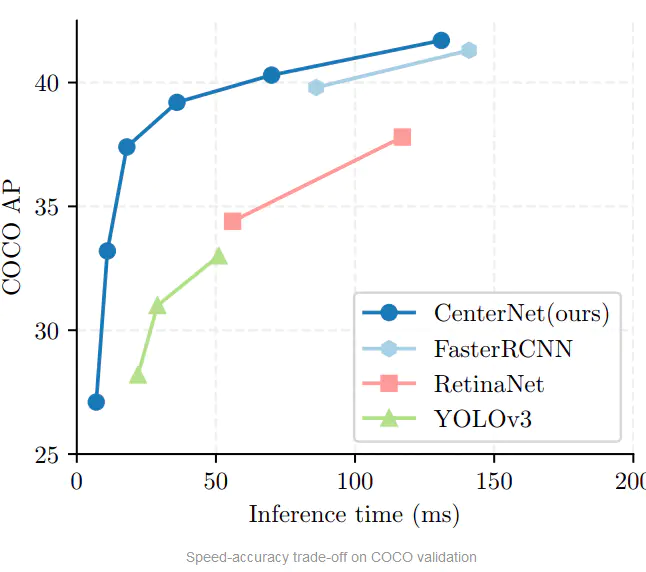
论文中提到:模型是端到端可微的,更简单,更快,更精确。Centernet的模型实现了速度和精确的很好权衡。
源码下载
https://github.com/bubbliiiing/centernet-tf2
喜欢的可以点个star噢。
Centernet实现思路
一、预测部分
1、主干网络介绍
Centernet用到的主干特征网络有多种,一般是以Hourglass Network、DLANet或者Resnet为主干特征提取网络,由于centernet所用到的Hourglass Network参数量太大,有19000W参数,DLANet并没有keras资源,本文以Resnet为例子进行解析。
ResNet50有两个基本的块,分别名为Conv Block和Identity Block,其中Conv Block输入和输出的维度是不一样的,所以不能连续串联,它的作用是改变网络的维度;Identity Block输入维度和输出维度相同,可以串联,用于加深网络的。
Conv Block的结构如下: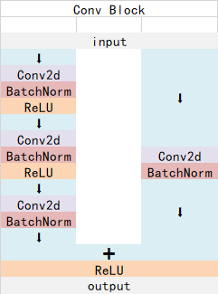
Identity Block的结构如下: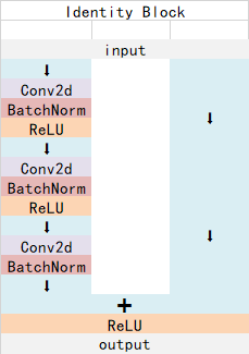
这两个都是残差网络结构。
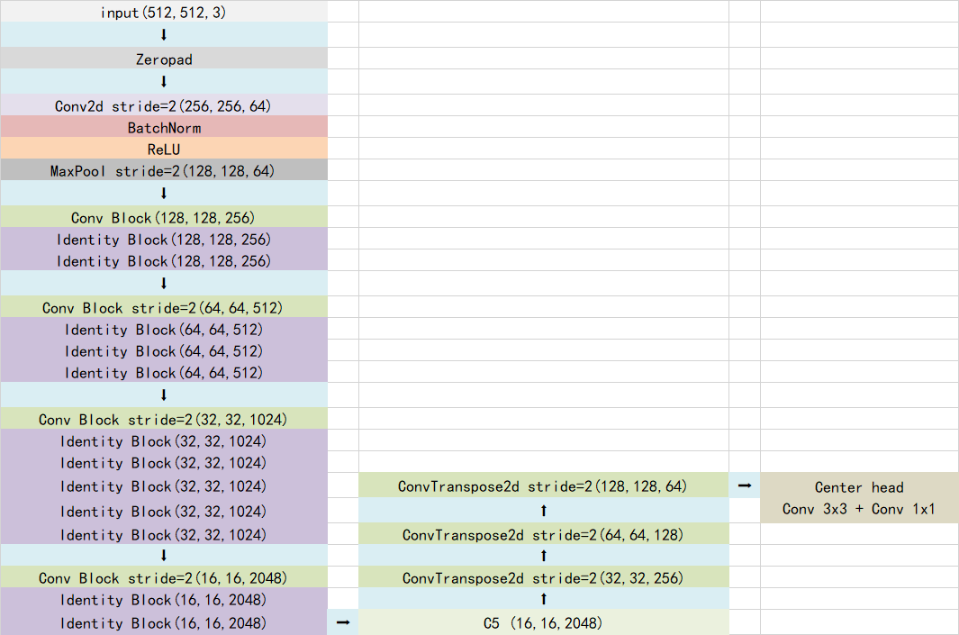
当我们输入的图片是512x512x3的时候,整体的特征层shape变化为: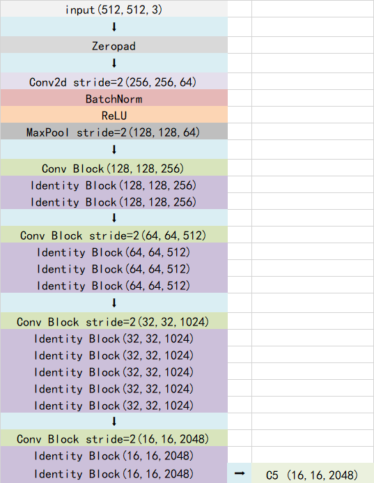
我们取出最终一个block的输出进行下一步的处理。也就是图上的C5,它的shape为16x16x2048。利用主干特征提取网络,我们获取到了一个初步的特征层,其shape为16x16x2048。
#-------------------------------------------------------------## ResNet50的网络部分#-------------------------------------------------------------#import numpy as npimport tensorflow.keras.backend as Kfrom tensorflow.keras import layersfrom tensorflow.keras.layers import (Activation, AveragePooling2D,BatchNormalization, Conv2D,Conv2DTranspose, Dense, Dropout, Flatten,Input, MaxPooling2D, ZeroPadding2D)from tensorflow.keras.models import Modelfrom tensorflow.keras.preprocessing import imagefrom tensorflow.keras.regularizers import l2def identity_block(input_tensor, kernel_size, filters, stage, block):filters1, filters2, filters3 = filtersconv_name_base = 'res' + str(stage) + block + '_branch'bn_name_base = 'bn' + str(stage) + block + '_branch'x = Conv2D(filters1, (1, 1), name=conv_name_base + '2a', use_bias=False)(input_tensor)x = BatchNormalization(name=bn_name_base + '2a')(x)x = Activation('relu')(x)x = Conv2D(filters2, kernel_size,padding='same', name=conv_name_base + '2b', use_bias=False)(x)x = BatchNormalization(name=bn_name_base + '2b')(x)x = Activation('relu')(x)x = Conv2D(filters3, (1, 1), name=conv_name_base + '2c', use_bias=False)(x)x = BatchNormalization(name=bn_name_base + '2c')(x)x = layers.add([x, input_tensor])x = Activation('relu')(x)return xdef conv_block(input_tensor, kernel_size, filters, stage, block, strides=(2, 2)):filters1, filters2, filters3 = filtersconv_name_base = 'res' + str(stage) + block + '_branch'bn_name_base = 'bn' + str(stage) + block + '_branch'x = Conv2D(filters1, (1, 1), strides=strides,name=conv_name_base + '2a', use_bias=False)(input_tensor)x = BatchNormalization(name=bn_name_base + '2a')(x)x = Activation('relu')(x)x = Conv2D(filters2, kernel_size, padding='same',name=conv_name_base + '2b', use_bias=False)(x)x = BatchNormalization(name=bn_name_base + '2b')(x)x = Activation('relu')(x)x = Conv2D(filters3, (1, 1), name=conv_name_base + '2c', use_bias=False)(x)x = BatchNormalization(name=bn_name_base + '2c')(x)shortcut = Conv2D(filters3, (1, 1), strides=strides,name=conv_name_base + '1', use_bias=False)(input_tensor)shortcut = BatchNormalization(name=bn_name_base + '1')(shortcut)x = layers.add([x, shortcut])x = Activation('relu')(x)return xdef ResNet50(inputs):# 512x512x3x = ZeroPadding2D((3, 3))(inputs)# 256,256,64x = Conv2D(64, (7, 7), strides=(2, 2), name='conv1', use_bias=False)(x)x = BatchNormalization(name='bn_conv1')(x)x = Activation('relu')(x)# 256,256,64 -> 128,128,64x = MaxPooling2D((3, 3), strides=(2, 2), padding="same")(x)# 128,128,64 -> 128,128,256x = conv_block(x, 3, [64, 64, 256], stage=2, block='a', strides=(1, 1))x = identity_block(x, 3, [64, 64, 256], stage=2, block='b')x = identity_block(x, 3, [64, 64, 256], stage=2, block='c')# 128,128,256 -> 64,64,512x = conv_block(x, 3, [128, 128, 512], stage=3, block='a')x = identity_block(x, 3, [128, 128, 512], stage=3, block='b')x = identity_block(x, 3, [128, 128, 512], stage=3, block='c')x = identity_block(x, 3, [128, 128, 512], stage=3, block='d')# 64,64,512 -> 32,32,1024x = conv_block(x, 3, [256, 256, 1024], stage=4, block='a')x = identity_block(x, 3, [256, 256, 1024], stage=4, block='b')x = identity_block(x, 3, [256, 256, 1024], stage=4, block='c')x = identity_block(x, 3, [256, 256, 1024], stage=4, block='d')x = identity_block(x, 3, [256, 256, 1024], stage=4, block='e')x = identity_block(x, 3, [256, 256, 1024], stage=4, block='f')# 32,32,1024 -> 16,16,2048x = conv_block(x, 3, [512, 512, 2048], stage=5, block='a')x = identity_block(x, 3, [512, 512, 2048], stage=5, block='b')x = identity_block(x, 3, [512, 512, 2048], stage=5, block='c')return x
2、利用初步特征获得高分辨率特征图
利用上一步获得到的resnet50的最后一个特征层的shape为(16,16,2048)。
对于该特征层,centernet利用三次反卷积进行上采样,从而更高的分辨率输出。为了节省计算量,这3个反卷积的输出通道数分别为256,128,64。
每一次反卷积,特征层的高和宽会变为原来的两倍,因此,在进行三次反卷积上采样后,我们获得的特征层的高和宽变为原来的8倍,此时特征层的高和宽为128x128,通道数为64。
此时我们获得了一个128x128x64的有效特征层(高分辨率特征图),我们会利用该有效特征层获得最终的预测结果。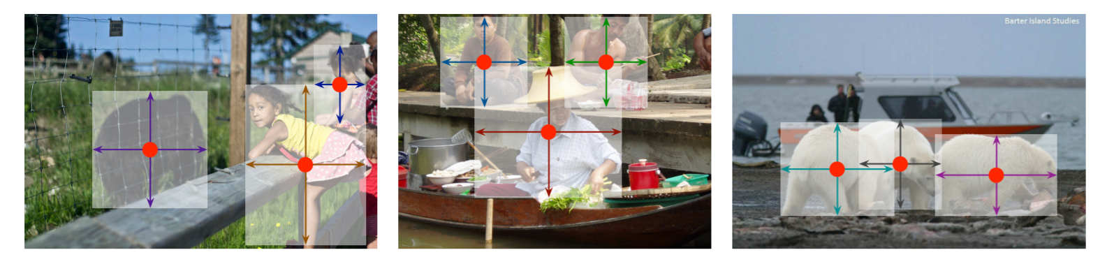
实现代码如下:
x = Dropout(rate=0.5)(x)#-------------------------------## 解码器#-------------------------------#num_filters = 256# 16, 16, 2048 -> 32, 32, 256 -> 64, 64, 128 -> 128, 128, 64for i in range(3):# 进行上采样x = Conv2DTranspose(num_filters // pow(2, i), (4, 4), strides=2, use_bias=False, padding='same',kernel_initializer='he_normal',kernel_regularizer=l2(5e-4))(x)x = BatchNormalization()(x)x = Activation('relu')(x)
3、Center Head从特征获取预测结果
通过上一步我们可以获得一个128x128x64的高分辨率特征图。
这个特征层相当于将整个图片划分成128x128个区域,每个区域存在一个特征点,如果某个物体的中心落在这个区域,那么就由这个特征点来确定。
(某个物体的中心落在这个区域,则由这个区域左上角的特征点来约定)
我们可以利用这个特征层进行三个卷积,分别是:
1、热力图预测,此时卷积的通道数为num_classes,最终结果为(128,128,num_classes),代表每一个热力点是否有物体存在,以及物体的种类;
2、中心点预测,此时卷积的通道数为2,最终结果为(128,128,2),代表每一个物体中心距离热力点偏移的情况;
3、宽高预测,此时卷积的通道数为2,最终结果为(128,128,2),代表每一个物体宽高的预测情况;
实现代码为:
def centernet_head(x,num_classes):x = Dropout(rate=0.5)(x)#-------------------------------## 解码器#-------------------------------#num_filters = 256# 16, 16, 2048 -> 32, 32, 256 -> 64, 64, 128 -> 128, 128, 64for i in range(3):# 进行上采样x = Conv2DTranspose(num_filters // pow(2, i), (4, 4), strides=2, use_bias=False, padding='same',kernel_initializer='he_normal',kernel_regularizer=l2(5e-4))(x)x = BatchNormalization()(x)x = Activation('relu')(x)# 最终获得128,128,64的特征层# hm headery1 = Conv2D(64, 3, padding='same', use_bias=False, kernel_initializer='he_normal', kernel_regularizer=l2(5e-4))(x)y1 = BatchNormalization()(y1)y1 = Activation('relu')(y1)y1 = Conv2D(num_classes, 1, kernel_initializer='he_normal', kernel_regularizer=l2(5e-4), activation='sigmoid')(y1)# wh headery2 = Conv2D(64, 3, padding='same', use_bias=False, kernel_initializer='he_normal', kernel_regularizer=l2(5e-4))(x)y2 = BatchNormalization()(y2)y2 = Activation('relu')(y2)y2 = Conv2D(2, 1, kernel_initializer='he_normal', kernel_regularizer=l2(5e-4))(y2)# reg headery3 = Conv2D(64, 3, padding='same', use_bias=False, kernel_initializer='he_normal', kernel_regularizer=l2(5e-4))(x)y3 = BatchNormalization()(y3)y3 = Activation('relu')(y3)y3 = Conv2D(2, 1, kernel_initializer='he_normal', kernel_regularizer=l2(5e-4))(y3)return y1, y2, y3
4、预测结果的解码
在对预测结果进行解码之前,我们再来看看预测结果代表了什么,预测结果可以分为3个部分:
1、heatmap热力图预测,此时卷积的通道数为num_classes,最终结果为(128,128,num_classes),代表每一个热力点是否有物体存在,以及物体的种类,最后一维度num_classes中的预测值代表属于每一个类的概率;
2、reg中心点预测,此时卷积的通道数为2,最终结果为(128,128,2),代表每一个物体中心距离热力点偏移的情况,最后一维度2中的预测值代表当前这个特征点向右下角偏移的情况;
3、wh宽高预测,此时卷积的通道数为2,最终结果为(128,128,2),代表每一个物体宽高的预测情况,最后一维度2中的预测值代表当前这个特征点对应的预测框的宽高;
特征层相当于将图像划分成128x128个特征点每个特征点负责预测中心落在其右下角一片区域的物体。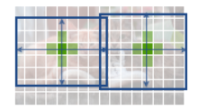
如图所示,蓝色的点为128x128的特征点,此时我们对左图红色的三个点进行解码操作演示:
1、进行中心点偏移,利用reg中心点预测对特征点坐标进行偏移,左图红色的三个特征点偏移后是右图橙色的三个点;
2、利用中心点加上和减去 wh宽高预测结果除以2,获得预测框的左上角和右下角。
3、此时获得的预测框就可以绘制在图片上了。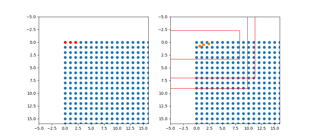
除去这样的解码操作,还有非极大抑制的操作需要进行,防止同一种类的框的堆积。
在论文中所说,centernet不像其它目标检测算法,在解码之后需要进行非极大抑制,centernet的非极大抑制在解码之前进行。采用的方法是最大池化,利用3x3的池化核在热力图上搜索,然后只保留一定区域内得分最大的框。
在实际使用时发现,当目标为小目标时,确实可以不在解码之后进行非极大抑制的后处理,如果目标为大目标,网络无法正确判断目标的中心时,还是需要进行非击大抑制的后处理的。
def nms(heat, kernel=3):hmax = MaxPooling2D((kernel, kernel), strides=1, padding='SAME')(heat)heat = tf.where(tf.equal(hmax, heat), heat, tf.zeros_like(heat))return heatdef topk(hm, max_objects=100):# hm -> Hot map热力图# 进行热力图的非极大抑制,利用3x3的卷积对热力图进行Max筛选,找出值最大的hm = nms(hm)# (b, h * w * c)b, h, w, c = tf.shape(hm)[0], tf.shape(hm)[1], tf.shape(hm)[2], tf.shape(hm)[3]# 将所有结果平铺,获得(b, h * w * c)hm = tf.reshape(hm, (b, -1))# (b, k), (b, k)scores, indices = tf.math.top_k(hm, k=max_objects, sorted=True)# 计算求出网格点,类别class_ids = indices % cxs = indices // c % wys = indices // c // windices = ys * w + xsreturn scores, indices, class_ids, xs, ysdef decode(hm, wh, reg, max_objects=100,num_classes=20):scores, indices, class_ids, xs, ys = topk(hm, max_objects=max_objects)# 获得batch_sizeb = tf.shape(hm)[0]# (b, h * w, 2)reg = tf.reshape(reg, [b, -1, 2])# (b, h * w, 2)wh = tf.reshape(wh, [b, -1, 2])length = tf.shape(wh)[1]# 找到其在1维上的索引batch_idx = tf.expand_dims(tf.range(0, b), 1)batch_idx = tf.tile(batch_idx, (1, max_objects))full_indices = tf.reshape(batch_idx, [-1]) * tf.to_int32(length) + tf.reshape(indices, [-1])# 取出top_k个框对应的参数topk_reg = tf.gather(tf.reshape(reg, [-1,2]), full_indices)topk_reg = tf.reshape(topk_reg, [b, -1, 2])topk_wh = tf.gather(tf.reshape(wh, [-1,2]), full_indices)topk_wh = tf.reshape(topk_wh, [b, -1, 2])# 计算调整后的中心topk_cx = tf.cast(tf.expand_dims(xs, axis=-1), tf.float32) + topk_reg[..., 0:1]topk_cy = tf.cast(tf.expand_dims(ys, axis=-1), tf.float32) + topk_reg[..., 1:2]# (b,k,1) (b,k,1)topk_x1, topk_y1 = topk_cx - topk_wh[..., 0:1] / 2, topk_cy - topk_wh[..., 1:2] / 2# (b,k,1) (b,k,1)topk_x2, topk_y2 = topk_cx + topk_wh[..., 0:1] / 2, topk_cy + topk_wh[..., 1:2] / 2# (b,k,1)scores = tf.expand_dims(scores, axis=-1)# (b,k,1)class_ids = tf.cast(tf.expand_dims(class_ids, axis=-1), tf.float32)# (b,k,6)detections = tf.concat([topk_x1, topk_y1, topk_x2, topk_y2, scores, class_ids], axis=-1)return detections
5、在原图上进行绘制
通过第三步,我们可以获得预测框在原图上的位置,而且这些预测框都是经过筛选的。这些筛选后的框可以直接绘制在图片上,就可以获得结果了。
二、训练部分
1、真实框的处理
既然在centernet中,物体的中心落在哪个特征点的右下角就由哪个特征点来负责预测,那么在训练的时候我们就需要找到真实框和特征点之间的关系。
真实框和特征点之间的关系,对应方式如下:
1、找到真实框的中心,通过真实框的中心找到其对应的特征点。
2、根据该真实框的种类,对网络应该有的热力图进行设置,即heatmap热力图。其实就是将对应的特征点里面的对应的种类,它的中心值设置为1,然后这个特征点附近的其它特征点中该种类对应的值按照高斯分布不断下降。
3、除去heatmap热力图外,还需要设置特征点对应的reg中心点和wh宽高,在找到真实框对应的特征点后,还需要设置该特征点对应的reg中心和wh宽高。这里的reg中心和wh宽高都是对于128x128的特征层的。
4、在获得网络应该有的预测结果后,就可以将预测结果和应该有的预测结果进行对比,对网络进行反向梯度调整了。
实现代码如下:
import mathfrom random import shuffleimport cv2import numpy as npfrom PIL import Imagefrom tensorflow import kerasfrom utils.utils import cvtColor, preprocess_inputdef draw_gaussian(heatmap, center, radius, k=1):diameter = 2 * radius + 1gaussian = gaussian2D((diameter, diameter), sigma=diameter / 6)x, y = int(center[0]), int(center[1])height, width = heatmap.shape[0:2]left, right = min(x, radius), min(width - x, radius + 1)top, bottom = min(y, radius), min(height - y, radius + 1)masked_heatmap = heatmap[y - top:y + bottom, x - left:x + right]masked_gaussian = gaussian[radius - top:radius + bottom, radius - left:radius + right]if min(masked_gaussian.shape) > 0 and min(masked_heatmap.shape) > 0: # TODO debugnp.maximum(masked_heatmap, masked_gaussian * k, out=masked_heatmap)return heatmapdef gaussian2D(shape, sigma=1):m, n = [(ss - 1.) / 2. for ss in shape]y, x = np.ogrid[-m:m + 1, -n:n + 1]h = np.exp(-(x * x + y * y) / (2 * sigma * sigma))h[h < np.finfo(h.dtype).eps * h.max()] = 0return hdef gaussian_radius(det_size, min_overlap=0.7):height, width = det_sizea1 = 1b1 = (height + width)c1 = width * height * (1 - min_overlap) / (1 + min_overlap)sq1 = np.sqrt(b1 ** 2 - 4 * a1 * c1)r1 = (b1 + sq1) / 2a2 = 4b2 = 2 * (height + width)c2 = (1 - min_overlap) * width * heightsq2 = np.sqrt(b2 ** 2 - 4 * a2 * c2)r2 = (b2 + sq2) / 2a3 = 4 * min_overlapb3 = -2 * min_overlap * (height + width)c3 = (min_overlap - 1) * width * heightsq3 = np.sqrt(b3 ** 2 - 4 * a3 * c3)r3 = (b3 + sq3) / 2return min(r1, r2, r3)class CenternetDatasets(keras.utils.Sequence):def __init__(self, annotation_lines, input_shape, batch_size, num_classes, train, max_objects = 100):self.annotation_lines = annotation_linesself.length = len(self.annotation_lines)self.input_shape = input_shapeself.output_shape = (int(input_shape[0]/4), int(input_shape[1]/4))self.batch_size = batch_sizeself.num_classes = num_classesself.train = trainself.max_objects = max_objectsdef __len__(self):return math.ceil(len(self.annotation_lines) / float(self.batch_size))def __getitem__(self, index):batch_images = np.zeros((self.batch_size, self.input_shape[0], self.input_shape[1], 3), dtype=np.float32)batch_hms = np.zeros((self.batch_size, self.output_shape[0], self.output_shape[1], self.num_classes), dtype=np.float32)batch_whs = np.zeros((self.batch_size, self.max_objects, 2), dtype=np.float32)batch_regs = np.zeros((self.batch_size, self.max_objects, 2), dtype=np.float32)batch_reg_masks = np.zeros((self.batch_size, self.max_objects), dtype=np.float32)batch_indices = np.zeros((self.batch_size, self.max_objects), dtype=np.float32)for b, i in enumerate(range(index * self.batch_size, (index + 1) * self.batch_size)):i = i % self.length#---------------------------------------------------## 训练时进行数据的随机增强# 验证时不进行数据的随机增强#---------------------------------------------------#image, box = self.get_random_data(self.annotation_lines[i], self.input_shape, random = self.train)if len(box) != 0:boxes = np.array(box[:, :4],dtype=np.float32)boxes[:, [0, 2]] = np.clip(boxes[:, [0, 2]] / self.input_shape[1] * self.output_shape[1], 0, self.output_shape[1] - 1)boxes[:, [1, 3]] = np.clip(boxes[:, [1, 3]] / self.input_shape[0] * self.output_shape[0], 0, self.output_shape[0] - 1)for i in range(len(box)):bbox = boxes[i].copy()cls_id = int(box[i, -1])h, w = bbox[3] - bbox[1], bbox[2] - bbox[0]if h > 0 and w > 0:radius = gaussian_radius((math.ceil(h), math.ceil(w)))radius = max(0, int(radius))#-------------------------------------------------## 计算真实框所属的特征点#-------------------------------------------------#ct = np.array([(bbox[0] + bbox[2]) / 2, (bbox[1] + bbox[3]) / 2], dtype=np.float32)ct_int = ct.astype(np.int32)#----------------------------## 绘制高斯热力图#----------------------------#batch_hms[b, :, :, cls_id] = draw_gaussian(batch_hms[b, :, :, cls_id], ct_int, radius)#---------------------------------------------------## 计算宽高真实值#---------------------------------------------------#batch_whs[b, i] = 1. * w, 1. * h#---------------------------------------------------## 计算中心偏移量#---------------------------------------------------#batch_regs[b, i] = ct - ct_int#---------------------------------------------------## 将对应的mask设置为1,用于排除多余的0#---------------------------------------------------#batch_reg_masks[b, i] = 1#---------------------------------------------------## 表示第ct_int[1]行的第ct_int[0]个。#---------------------------------------------------#batch_indices[b, i] = ct_int[1] * self.output_shape[0] + ct_int[0]batch_images[b] = preprocess_input(image)return [batch_images, batch_hms, batch_whs, batch_regs, batch_reg_masks, batch_indices], np.zeros((self.batch_size,))def generate(self):i = 0while True:batch_images = np.zeros((self.batch_size, self.input_shape[0], self.input_shape[1], 3), dtype=np.float32)batch_hms = np.zeros((self.batch_size, self.output_shape[0], self.output_shape[1], self.num_classes), dtype=np.float32)batch_whs = np.zeros((self.batch_size, self.max_objects, 2), dtype=np.float32)batch_regs = np.zeros((self.batch_size, self.max_objects, 2), dtype=np.float32)batch_reg_masks = np.zeros((self.batch_size, self.max_objects), dtype=np.float32)batch_indices = np.zeros((self.batch_size, self.max_objects), dtype=np.float32)for b in range(self.batch_size):#---------------------------------------------------## 训练时进行数据的随机增强# 验证时不进行数据的随机增强#---------------------------------------------------#image, box = self.get_random_data(self.annotation_lines[i], self.input_shape, random = self.train)if len(box) != 0:boxes = np.array(box[:, :4],dtype=np.float32)boxes[:, [0, 2]] = np.clip(boxes[:, [0, 2]] / self.input_shape[1] * self.output_shape[1], 0, self.output_shape[1] - 1)boxes[:, [1, 3]] = np.clip(boxes[:, [1, 3]] / self.input_shape[0] * self.output_shape[0], 0, self.output_shape[0] - 1)for i in range(len(box)):bbox = boxes[i].copy()cls_id = int(box[i, -1])h, w = bbox[3] - bbox[1], bbox[2] - bbox[0]if h > 0 and w > 0:radius = gaussian_radius((math.ceil(h), math.ceil(w)))radius = max(0, int(radius))#-------------------------------------------------## 计算真实框所属的特征点#-------------------------------------------------#ct = np.array([(bbox[0] + bbox[2]) / 2, (bbox[1] + bbox[3]) / 2], dtype=np.float32)ct_int = ct.astype(np.int32)#----------------------------## 绘制高斯热力图#----------------------------#batch_hms[b, :, :, cls_id] = draw_gaussian(batch_hms[b, :, :, cls_id], ct_int, radius)#---------------------------------------------------## 计算宽高真实值#---------------------------------------------------#batch_whs[b, i] = 1. * w, 1. * h#---------------------------------------------------## 计算中心偏移量#---------------------------------------------------#batch_regs[b, i] = ct - ct_int#---------------------------------------------------## 将对应的mask设置为1,用于排除多余的0#---------------------------------------------------#batch_reg_masks[b, i] = 1#---------------------------------------------------## 表示第ct_int[1]行的第ct_int[0]个。#---------------------------------------------------#batch_indices[b, i] = ct_int[1] * self.output_shape[0] + ct_int[0]batch_images[b] = preprocess_input(image)yield batch_images, batch_hms, batch_whs, batch_regs, batch_reg_masks, batch_indicesdef rand(self, a=0, b=1):return np.random.rand()*(b-a) + adef get_random_data(self, annotation_line, input_shape, jitter=.3, hue=.1, sat=1.5, val=1.5, random=True):line = annotation_line.split()#------------------------------## 读取图像并转换成RGB图像#------------------------------#image = Image.open(line[0])image = cvtColor(image)#------------------------------## 获得图像的高宽与目标高宽#------------------------------#iw, ih = image.sizeh, w = input_shape#------------------------------## 获得预测框#------------------------------#box = np.array([np.array(list(map(int,box.split(',')))) for box in line[1:]])if not random:scale = min(w/iw, h/ih)nw = int(iw*scale)nh = int(ih*scale)dx = (w-nw)//2dy = (h-nh)//2#---------------------------------## 将图像多余的部分加上灰条#---------------------------------#image = image.resize((nw,nh), Image.BICUBIC)new_image = Image.new('RGB', (w,h), (128,128,128))new_image.paste(image, (dx, dy))image_data = np.array(new_image, np.float32)#---------------------------------## 对真实框进行调整#---------------------------------#if len(box)>0:np.random.shuffle(box)box[:, [0,2]] = box[:, [0,2]]*nw/iw + dxbox[:, [1,3]] = box[:, [1,3]]*nh/ih + dybox[:, 0:2][box[:, 0:2]<0] = 0box[:, 2][box[:, 2]>w] = wbox[:, 3][box[:, 3]>h] = hbox_w = box[:, 2] - box[:, 0]box_h = box[:, 3] - box[:, 1]box = box[np.logical_and(box_w>1, box_h>1)] # discard invalid boxreturn image_data, box#------------------------------------------## 对图像进行缩放并且进行长和宽的扭曲#------------------------------------------#new_ar = w/h * self.rand(1-jitter,1+jitter) / self.rand(1-jitter,1+jitter)scale = self.rand(.25, 2)if new_ar < 1:nh = int(scale*h)nw = int(nh*new_ar)else:nw = int(scale*w)nh = int(nw/new_ar)image = image.resize((nw,nh), Image.BICUBIC)#------------------------------------------## 将图像多余的部分加上灰条#------------------------------------------#dx = int(self.rand(0, w-nw))dy = int(self.rand(0, h-nh))new_image = Image.new('RGB', (w,h), (128,128,128))new_image.paste(image, (dx, dy))image = new_image#------------------------------------------## 翻转图像#------------------------------------------#flip = self.rand()<.5if flip: image = image.transpose(Image.FLIP_LEFT_RIGHT)#------------------------------------------## 色域扭曲#------------------------------------------#hue = self.rand(-hue, hue)sat = self.rand(1, sat) if self.rand()<.5 else 1/self.rand(1, sat)val = self.rand(1, val) if self.rand()<.5 else 1/self.rand(1, val)x = cv2.cvtColor(np.array(image,np.float32)/255, cv2.COLOR_RGB2HSV)x[..., 0] += hue*360x[..., 0][x[..., 0]>1] -= 1x[..., 0][x[..., 0]<0] += 1x[..., 1] *= satx[..., 2] *= valx[x[:,:, 0]>360, 0] = 360x[:, :, 1:][x[:, :, 1:]>1] = 1x[x<0] = 0image_data = cv2.cvtColor(x, cv2.COLOR_HSV2RGB)*255 # numpy array, 0 to 1#---------------------------------## 对真实框进行调整#---------------------------------#if len(box)>0:np.random.shuffle(box)box[:, [0,2]] = box[:, [0,2]]*nw/iw + dxbox[:, [1,3]] = box[:, [1,3]]*nh/ih + dyif flip: box[:, [0,2]] = w - box[:, [2,0]]box[:, 0:2][box[:, 0:2]<0] = 0box[:, 2][box[:, 2]>w] = wbox[:, 3][box[:, 3]>h] = hbox_w = box[:, 2] - box[:, 0]box_h = box[:, 3] - box[:, 1]box = box[np.logical_and(box_w>1, box_h>1)]return image_data, boxdef on_epoch_begin(self):shuffle(self.annotation_lines)
2、利用处理完的真实框与对应图片的预测结果计算loss
loss计算分为三个部分,分别是:
1、热力图的loss
2、reg中心点的loss
3、wh宽高的loss
具体情况如下:
1、热力图的loss采用focal loss的思想进行运算,其中 α 和 β 是Focal Loss的超参数,而其中的N是正样本的数量,用于进行标准化。 α 和 β在这篇论文中和分别是2和4。
整体思想和Focal Loss类似,对于容易分类的样本,适当减少其训练比重也就是loss值。
在公式中,带帽子的Y是预测值,不戴帽子的Y是真实值。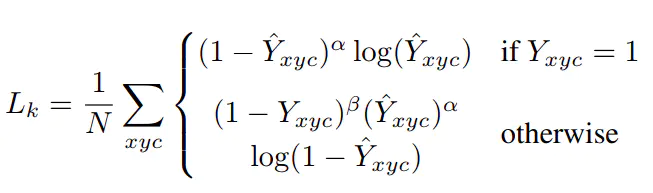
2、reg中心点的loss和wh宽高的loss使用的是普通L1损失函数
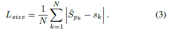
reg中心点预测和wh宽高预测都直接采用了特征层坐标的尺寸,也就是在0到128之内。
由于wh宽高预测的loss会比较大,其loss乘上了一个系数,论文是0.1。
reg中心点预测的系数则为1。
总的loss就变成了: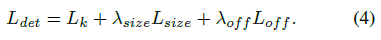
实现代码如下:
def focal_loss(hm_pred, hm_true):# 找到正样本和负样本pos_mask = tf.cast(tf.equal(hm_true, 1), tf.float32)# 小于1的都是负样本neg_mask = tf.cast(tf.less(hm_true, 1), tf.float32)neg_weights = tf.pow(1 - hm_true, 4)pos_loss = -tf.log(tf.clip_by_value(hm_pred, 1e-7, 1.)) * tf.pow(1 - hm_pred, 2) * pos_maskneg_loss = -tf.log(tf.clip_by_value(1 - hm_pred, 1e-7, 1.)) * tf.pow(hm_pred, 2) * neg_weights * neg_masknum_pos = tf.reduce_sum(pos_mask)pos_loss = tf.reduce_sum(pos_loss)neg_loss = tf.reduce_sum(neg_loss)cls_loss = tf.cond(tf.greater(num_pos, 0), lambda: (pos_loss + neg_loss) / num_pos, lambda: neg_loss)return cls_lossdef reg_l1_loss(y_pred, y_true, indices, mask):b, c = tf.shape(y_pred)[0], tf.shape(y_pred)[-1]k = tf.shape(indices)[1]y_pred = tf.reshape(y_pred, (b, -1, c))length = tf.shape(y_pred)[1]indices = tf.cast(indices, tf.int32)# 找到其在1维上的索引batch_idx = tf.expand_dims(tf.range(0, b), 1)batch_idx = tf.tile(batch_idx, (1, k))full_indices = (tf.reshape(batch_idx, [-1]) * tf.to_int32(length) +tf.reshape(indices, [-1]))# 取出对应的预测值y_pred = tf.gather(tf.reshape(y_pred, [-1,c]),full_indices)y_pred = tf.reshape(y_pred, [b, -1, c])mask = tf.tile(tf.expand_dims(mask, axis=-1), (1, 1, 2))# 求取l1损失值total_loss = tf.reduce_sum(tf.abs(y_true * mask - y_pred * mask))reg_loss = total_loss / (tf.reduce_sum(mask) + 1e-4)return reg_lossdef loss(args):#-----------------------------------------------------------------------------------------------------------------## hm_pred:热力图的预测值 (self.batch_size, self.output_size[0], self.output_size[1], self.num_classes)# wh_pred:宽高的预测值 (self.batch_size, self.output_size[0], self.output_size[1], 2)# reg_pred:中心坐标偏移预测值 (self.batch_size, self.output_size[0], self.output_size[1], 2)# hm_true:热力图的真实值 (self.batch_size, self.output_size[0], self.output_size[1], self.num_classes)# wh_true:宽高的真实值 (self.batch_size, self.max_objects, 2)# reg_true:中心坐标偏移真实值 (self.batch_size, self.max_objects, 2)# reg_mask:真实值的mask (self.batch_size, self.max_objects)# indices:真实值对应的坐标 (self.batch_size, self.max_objects)#-----------------------------------------------------------------------------------------------------------------#hm_pred, wh_pred, reg_pred, hm_true, wh_true, reg_true, reg_mask, indices = argshm_loss = focal_loss(hm_pred, hm_true)wh_loss = 0.1 * reg_l1_loss(wh_pred, wh_true, indices, reg_mask)reg_loss = reg_l1_loss(reg_pred, reg_true, indices, reg_mask)total_loss = hm_loss + wh_loss + reg_loss# total_loss = tf.Print(total_loss,[hm_loss,wh_loss,reg_loss])return total_loss
训练自己的Centernet模型
首先前往Github下载对应的仓库,下载完后利用解压软件解压,之后用编程软件打开文件夹。
注意打开的根目录必须正确,否则相对目录不正确的情况下,代码将无法运行。
一定要注意打开后的根目录是文件存放的目录。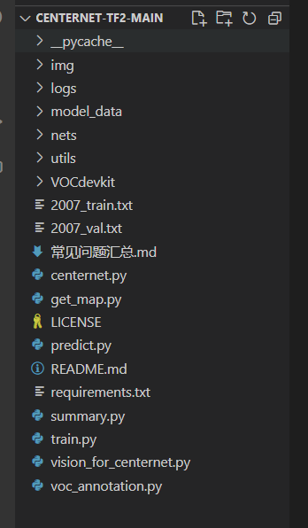
一、数据集的准备
本文使用VOC格式进行训练,训练前需要自己制作好数据集,如果没有自己的数据集,可以通过Github连接下载VOC12+07的数据集尝试下。
训练前将标签文件放在VOCdevkit文件夹下的VOC2007文件夹下的Annotation中。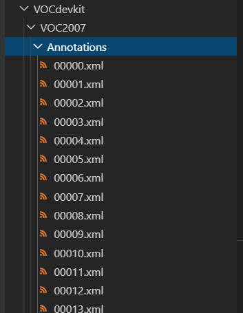
训练前将图片文件放在VOCdevkit文件夹下的VOC2007文件夹下的JPEGImages中。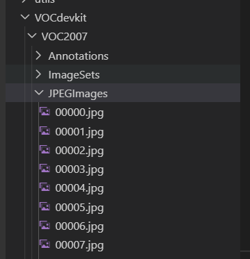
此时数据集的摆放已经结束。
二、数据集的处理
在完成数据集的摆放之后,我们需要对数据集进行下一步的处理,目的是获得训练用的2007_train.txt以及2007_val.txt,需要用到根目录下的voc_annotation.py。
voc_annotation.py里面有一些参数需要设置。
分别是annotation_mode、classes_path、trainval_percent、train_percent、VOCdevkit_path,第一次训练可以仅修改classes_path
'''annotation_mode用于指定该文件运行时计算的内容annotation_mode为0代表整个标签处理过程,包括获得VOCdevkit/VOC2007/ImageSets里面的txt以及训练用的2007_train.txt、2007_val.txtannotation_mode为1代表获得VOCdevkit/VOC2007/ImageSets里面的txtannotation_mode为2代表获得训练用的2007_train.txt、2007_val.txt'''annotation_mode = 0'''必须要修改,用于生成2007_train.txt、2007_val.txt的目标信息与训练和预测所用的classes_path一致即可如果生成的2007_train.txt里面没有目标信息那么就是因为classes没有设定正确仅在annotation_mode为0和2的时候有效'''classes_path = 'model_data/voc_classes.txt''''trainval_percent用于指定(训练集+验证集)与测试集的比例,默认情况下 (训练集+验证集):测试集 = 9:1train_percent用于指定(训练集+验证集)中训练集与验证集的比例,默认情况下 训练集:验证集 = 9:1仅在annotation_mode为0和1的时候有效'''trainval_percent = 0.9train_percent = 0.9'''指向VOC数据集所在的文件夹默认指向根目录下的VOC数据集'''VOCdevkit_path = 'VOCdevkit'
classes_path用于指向检测类别所对应的txt,以voc数据集为例,我们用的txt为: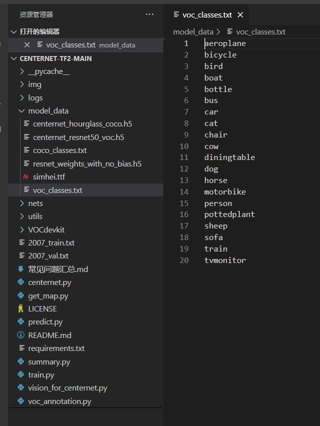
训练自己的数据集时,可以自己建立一个cls_classes.txt,里面写自己所需要区分的类别。
三、开始网络训练
通过voc_annotation.py我们已经生成了2007_train.txt以及2007_val.txt,此时我们可以开始训练了。
训练的参数较多,大家可以在下载库后仔细看注释,其中最重要的部分依然是train.py里的classes_path。
classes_path用于指向检测类别所对应的txt,这个txt和voc_annotation.py里面的txt一样!训练自己的数据集必须要修改!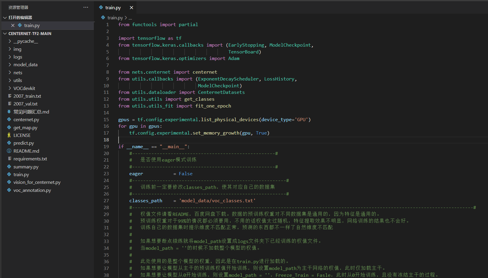
修改完classes_path后就可以运行train.py开始训练了,在训练多个epoch后,权值会生成在logs文件夹中。
其它参数的作用如下:
#----------------------------------------------------## 是否使用eager模式训练#----------------------------------------------------#eager = False#--------------------------------------------------------## 训练前一定要修改classes_path,使其对应自己的数据集#--------------------------------------------------------#classes_path = 'model_data/voc_classes.txt'#----------------------------------------------------------------------------------------------------------------------------## 权值文件请看README,百度网盘下载。数据的预训练权重对不同数据集是通用的,因为特征是通用的。# 预训练权重对于99%的情况都必须要用,不用的话权值太过随机,特征提取效果不明显,网络训练的结果也不会好。# 训练自己的数据集时提示维度不匹配正常,预测的东西都不一样了自然维度不匹配## 如果想要断点续练就将model_path设置成logs文件夹下已经训练的权值文件。# 当model_path = ''的时候不加载整个模型的权值。## 此处使用的是整个模型的权重,因此是在train.py进行加载的。# 如果想要让模型从主干的预训练权值开始训练,则设置model_path为主干网络的权值,此时仅加载主干。# 如果想要让模型从0开始训练,则设置model_path = '',Freeze_Train = Fasle,此时从0开始训练,且没有冻结主干的过程。# 一般来讲,从0开始训练效果会很差,因为权值太过随机,特征提取效果不明显。#----------------------------------------------------------------------------------------------------------------------------#model_path = 'model_data/centernet_resnet50_voc.h5'#------------------------------------------------------## 输入的shape大小,32的倍数#------------------------------------------------------#input_shape = [512, 512]#-------------------------------------------## 主干特征提取网络的选择# resnet50和hourglass#-------------------------------------------#backbone = "resnet50"#----------------------------------------------------## 训练分为两个阶段,分别是冻结阶段和解冻阶段。# 显存不足与数据集大小无关,提示显存不足请调小batch_size。# 受到BatchNorm层影响,batch_size最小为2,不能为1。#----------------------------------------------------##----------------------------------------------------## 冻结阶段训练参数# 此时模型的主干被冻结了,特征提取网络不发生改变# 占用的显存较小,仅对网络进行微调#----------------------------------------------------#Init_Epoch = 0Freeze_Epoch = 50Freeze_batch_size = 16Freeze_lr = 1e-3#----------------------------------------------------## 解冻阶段训练参数# 此时模型的主干不被冻结了,特征提取网络会发生改变# 占用的显存较大,网络所有的参数都会发生改变#----------------------------------------------------#UnFreeze_Epoch = 100Unfreeze_batch_size = 8Unfreeze_lr = 1e-4#------------------------------------------------------## 是否进行冻结训练,默认先冻结主干训练后解冻训练。#------------------------------------------------------#Freeze_Train = True#------------------------------------------------------## 用于设置是否使用多线程读取数据,0代表关闭多线程# 开启后会加快数据读取速度,但是会占用更多内存# keras里开启多线程有些时候速度反而慢了许多# 在IO为瓶颈的时候再开启多线程,即GPU运算速度远大于读取图片的速度。#------------------------------------------------------#num_workers = 0#----------------------------------------------------## 获得图片路径和标签#----------------------------------------------------#train_annotation_path = '2007_train.txt'val_annotation_path = '2007_val.txt'
四、训练结果预测
训练结果预测需要用到两个文件,分别是yolo.py和predict.py。
我们首先需要去yolo.py里面修改model_path以及classes_path,这两个参数必须要修改。
model_path指向训练好的权值文件,在logs文件夹里。
classes_path指向检测类别所对应的txt。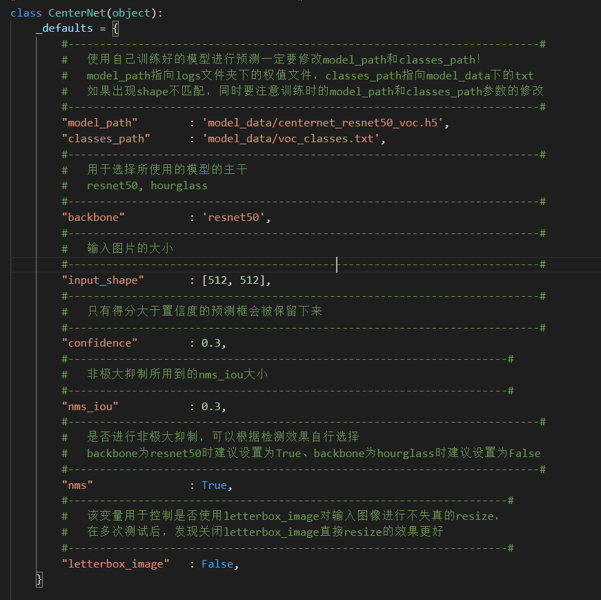
完成修改后就可以运行predict.py进行检测了。运行后输入图片路径即可检测。


:Docker 部署 Redis 以及相关配置信息")


还没有评论,来说两句吧...