hand crafted feature:histogram(直方图)
文章目录
- 直方图是什么
- 约定
- 灰度级
- 直方图的定义
- 直方图计算方法
- 素材
- 程序
- 计算结果
- 直方图的作用
- 作为图像特征
- 调整图像色彩
直方图是什么
约定
为了方便叙述,此处关于直方图概念的讨论做一些约束:
- 图像数据类型是uint8类型,可表达的数值范围是[0, 255]
- 以灰度图作为讨论的基础,此时的直方图可进一步称为灰度直方图
但是也应当悉知,当我们在上述约束下把直方图的概念讨论清楚后,相应的理论同样适用于其他数据类型,如float,也适用于彩色图像。
灰度级
我们可以把[0, 255]的范围划分为多个区间,每一个区间就称为一个灰度级。
特别的,当我们将[0, 255]平均划分为256个区间时,每一个数字就对应一个灰度级。
直方图的定义
直方图是图像每一个灰度级与该灰度级出现的概率的对应关系,由于灰度级是离散的,所以直方图是一个离散函数。假设一张图像的像素总数是 N N N,属于某个灰度级 g g g的像素总数是 N g N_g Ng,那么该灰度级出现的概率就是
P g = N g / N P_g = N_g / N Pg=Ng/N
此时,直方图的横坐标就是灰度级 g g g,而纵坐标就是概率 P g P_g Pg。
也可以将直方图纵坐标定义为 N g N_g Ng,即灰度级中的像素总数,但是这种定义不利于进一步的理论理解,比如直方图均衡化相关理论。但是程序计算的结果通常以像素数目这种定义方式返回。
直方图计算方法
素材
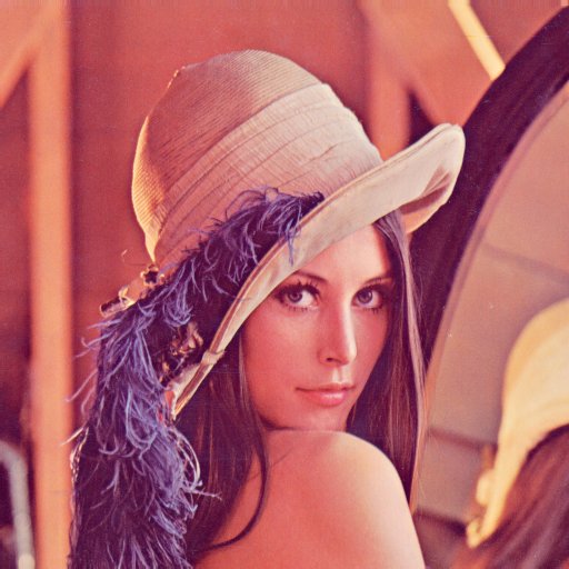
素材使用美女lena,图片下载网址:https://www.ece.rice.edu/~wakin/images/lena512color.tiff
程序
直方图的计算方法很简单,核心思想就是计数。
将待统计的像素值区域划分成一个个的区间(在计算直方图时我们一般把这样的区间称为bin),区间划分方式一般是等分(当然同学你真的想不等分也不是不可以),然后统计图像落在各个区间中的像素的数量即可得到直方图。
下面的程序使用两种方式计算直方图,一种是自己写的函数compute_histogram,另一种是opencv的库函数cv2.calcHist,我们可以进行对比验证,看看自写函数与opencv的库函数计算的结果是否一致。我已经验证了是一致的。吐槽一下,opencv库函数的入参形态有点怪异。。。
请注意,彩色图像的直方图应当对每个通道分别计算,而不是对所有通道一起计算。
计算程序如下,文件名保存为histogram.py
# -*- coding: utf-8 -*-import cv2import numpy as npdef compute_histogram(image, channel, hist_size=256, ranges=None):""" Description: ------------ compute histogram of image Inputs: ------- image: image data (ndarray) channel: channel of image to be computed hist_size: bins number of histogram ranges: data range to be counted Outputs: -------- hist: histogram of image for a certain channel """# check argumentsif ranges is None:ranges = [0, 256]assert hist_size > 1, 'hist_size must be greater than 1'assert image.ndim == 2 or image.ndim == 3, 'image dimension must be 2 or 3'if image.ndim == 3:assert channel < image.shape[2], \'channel must be less than image channels'image = image[:, :, channel]# compute histogrambin_width = (ranges[1] - ranges[0]) / hist_sizehist = np.zeros([hist_size])for i in range(hist_size):bin_beg = ranges[0] + i * bin_widthbin_end = ranges[0] + (i + 1) * bin_widthhist[i] = np.sum((image >= bin_beg) & (image < bin_end))return histdef normalize_histogram(hist):""" Description: ------------ normalize histogram by dividing sum of hist Inputs: ------- hist: histogram Outputs: -------- hist: normalized histogram """hist /= np.sum(hist)return histdef plot(hist, color, image_height, ratio):""" Description: ------------ plot histogram by 2D image Inputs: ------- hist: histogram color: color of histogram image image_height: height of histogram image ratio: max height of hist over image height Outputs: -------- hist_image: histogram image """image_width = hist.shape[0]if isinstance(color, (int, float)):hist_image = np.zeros([image_height, image_width], dtype=np.uint8)else:assert len(color) == 3, 'length of color must be 3 if it is not scalar'hist_image = np.zeros([image_height, image_width, 3], dtype=np.uint8)hist /= np.max(hist)for x in range(image_width):pt1 = (x, image_height)pt2 = (x, int(image_height - np.round(hist[x] * image_height * ratio)))cv2.line(hist_image, pt1, pt2, color=color)return hist_imagedef is_equal(hist_a, hist_b):""" Description: ------------ check whether two histograms are equal Inputs: ------- hist_a and hist_b are two histograms Outputs: -------- return True if two histograms are equal, and False if not """assert hist_a.ndim == hist_b.ndim == 1, 'hist must be rank-1 array'assert hist_a.shape[0] == hist_b.shape[0]return np.all(hist_a == hist_b)if __name__ == '__main__':# parametersHIST_SIZE = 256RANGES = [0, 256]HIST_IMAGE_HEIGHT = 256RATIO = 0.9# read imagescolor_image = cv2.imread('lena512color.tiff', cv2.IMREAD_UNCHANGED)gray_image = cv2.cvtColor(color_image, cv2.COLOR_BGR2GRAY)# gray imagehist_gray = compute_histogram(gray_image, 0, HIST_SIZE, RANGES)hist_gray_cv2 = cv2.calcHist([gray_image], channels=[0], mask=None,histSize=[HIST_SIZE], ranges=RANGES)hist_gray_cv2 = np.squeeze(hist_gray_cv2)print(is_equal(hist_gray, hist_gray_cv2))hist_gray_image = plot(hist_gray, color=255,image_height=HIST_IMAGE_HEIGHT, ratio=RATIO)# color imagehist_blue = compute_histogram(color_image, 0, HIST_SIZE, RANGES)hist_green = compute_histogram(color_image, 1, HIST_SIZE, RANGES)hist_red = compute_histogram(color_image, 2, HIST_SIZE, RANGES)hist_blue_cv2 = cv2.calcHist([color_image], channels=[0], mask=None,histSize=[HIST_SIZE], ranges=RANGES)hist_green_cv2 = cv2.calcHist([color_image], channels=[1], mask=None,histSize=[HIST_SIZE], ranges=RANGES)hist_red_cv2 = cv2.calcHist([color_image], channels=[2], mask=None,histSize=[HIST_SIZE], ranges=RANGES)hist_blue_cv2 = np.squeeze(hist_blue_cv2)hist_green_cv2 = np.squeeze(hist_green_cv2)hist_red_cv2 = np.squeeze(hist_red_cv2)print(is_equal(hist_blue, hist_blue_cv2),is_equal(hist_green, hist_green_cv2),is_equal(hist_red, hist_red_cv2))hist_blue_image = plot(hist_blue, color=(255, 0, 0),image_height=HIST_IMAGE_HEIGHT, ratio=RATIO)hist_green_image = plot(hist_green, color=(0, 255, 0),image_height=HIST_IMAGE_HEIGHT, ratio=RATIO)hist_red_image = plot(hist_red, color=(0, 0, 255),image_height=HIST_IMAGE_HEIGHT, ratio=RATIO)cv2.imwrite('lena_gray.png', gray_image)cv2.imwrite('hist_gray.png', hist_gray_image)cv2.imwrite('hist_blue.png', hist_blue_image)cv2.imwrite('hist_green.png', hist_green_image)cv2.imwrite('hist_red.png', hist_red_image)
上述程序将lena图转为灰度,然后计算了其直方图。而后又彩色的lena图分别计算了BGR三个通道的直方图。
计算结果
灰度图的直方图: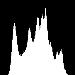
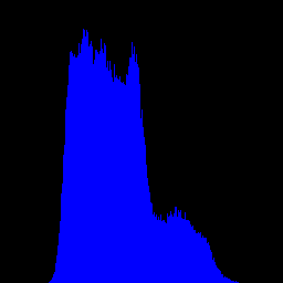
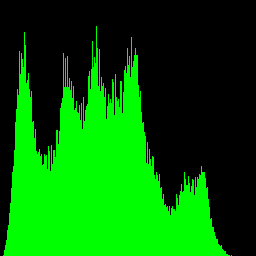
彩色图的直方图:
直方图的作用
作为图像特征
直方图可以用作图像特征,其特点如下:
- 是图像全局特征的表达
- 仅是图像色彩特征的表达
- 该特征的语义表达能力非常弱,或者换句直白点的话讲,这个特征比较挫
比如下面三张图,分别是ocean, sky1, sky2
ocean
sky1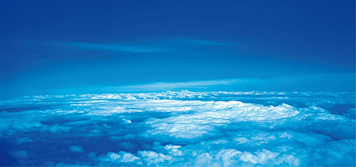
sky2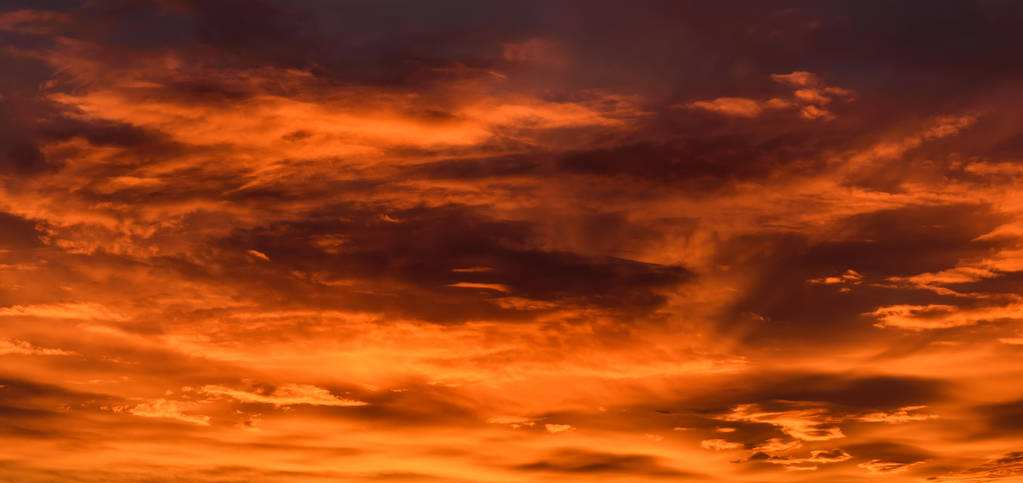
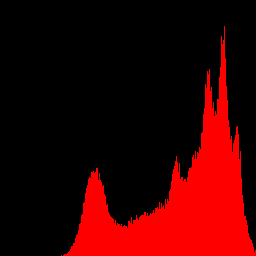
我们分别计算这三张图的直方图特征,计算方法是对BGR三个通道分别计算直方图,而后将其串联起来作为特征。然后发现,因为ocean和sky1的色彩比较相近,所以两者相似度较高;而sky1和sky2尽管都是天空(即语义相近),但是因为色彩相差较大,所以相似度反而很低。
计算代码如下:
# -*- coding: utf-8 -*-import cv2import numpy as npfrom histogram import compute_histogramHIST_SIZE = 128def cos_similarity(feature_a, feature_b):""" Description: ------------ compute cosine similarity of two features Inputs: ------- feature_a and feature_b are ndarrays with same shape Outputs: -------- cos_sim: cosine similarity """feature_a /= np.linalg.norm(feature_a)feature_b /= np.linalg.norm(feature_b)cos_sim = np.sum(feature_a * feature_b)return cos_simif __name__ == '__main__':image_sky1 = cv2.imread('sky1.png', cv2.IMREAD_UNCHANGED)image_sky2 = cv2.imread('sky2.png', cv2.IMREAD_UNCHANGED)image_ocean = cv2.imread('ocean.png', cv2.IMREAD_UNCHANGED)hist_sky1 = []hist_sky2 = []hist_ocean = []for ch in range(3):hist_sky1.append(compute_histogram(image_sky1, ch, HIST_SIZE))hist_sky2.append(compute_histogram(image_sky2, ch, HIST_SIZE))hist_ocean.append(compute_histogram(image_ocean, ch, HIST_SIZE))hist_sky1 = np.concatenate(hist_sky1)hist_sky2 = np.concatenate(hist_sky2)hist_ocean = np.concatenate(hist_ocean)sim_ocean_sky1 = cos_similarity(hist_sky1, hist_ocean)sim_sky1_sky2 = cos_similarity(hist_sky1, hist_sky2)print('cosine similarity of ocean vs sky: %0.4f' % sim_ocean_sky1)print('cosine similarity of sky1 vs sky2: %0.4f' % sim_sky1_sky2)
结果是:
cosine similarity of ocean vs sky: 0.7584cosine similarity of sky1 vs sky2: 0.0907
调整图像色彩
我们可以对图像中的各个像素进行灰度变换从而调整图像色彩。比如在诸如Photoshop之类的图像编辑软件中,可以看到如下图所示的功能:
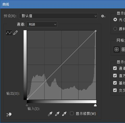
上图中横坐标是图像原始的灰度级,纵坐标是对图像进行一定的灰度变换后得到的灰度级,改变曲线就可以改变输入输出之间的灰度映射关系,如果对三个通道分别调整该曲线,就可以起到调整图像色彩的作用。需要注意的是,灰度变换本身并不需要计算直方图,而是只是需要对其进行观察。
此处不详细讨论,后面可以专门写一个灰度变换的主题。


")


还没有评论,来说两句吧...