【神经网络和深度学习】—— 从理论到实践深入理解RNN(Recurrent Neural Network) 基于Pytorch实现
文章目录
- 一、RNN的理论部分
- 1.1 Why Recurrent Neural Network
- 1.2 RNN 的工作原理解析
- 1.2.1 数据的定义部分
- 1.2.2 RNN 的具体运算过程
- 1.2.3 几种不同类型的 RNN
- 二、基于Pytorch的RNN实践部分
- 2.1 在Pytorch里面对 RNN 输入参数的认识
- 2.2 nn.RNN 里面的 forward 方法:
- Example:利用RNN进时间序列的预测
一、RNN的理论部分
1.1 Why Recurrent Neural Network
我们之前学习的 DNN,CNN。在某一些领域都取得了显著的成效(例如 CNN 在 CV 领域的卓越成绩)。但是他们都只能单独的取处理一个个的输入,前一个输入和后一个输入是完全没有关系的。但是,某些任务需要能够更好的处理序列的信息,即前面的输入和后面的输入是有关系的。
但是,当我们在理解一句话意思时,孤立的理解这句话的每个词是不够的,我们需要处理这些词连接起来的整个序列; 当我们处理视频的时候,我们也不能只单独的去分析每一帧,而要分析这些帧连接起来的整个序列。
所以为了解决一些这样类似的问题,能够更好的处理序列的信息,RNN就诞生了
1.2 RNN 的工作原理解析
1.2.1 数据的定义部分
首先,我们约定一个数学符号:我们用 x x x 表示输入的时间序列。举一个最常见的例子:如果我们需要进行文本人名的识别。我们将会给 RNN 输入这样一个时间序列 x x x: H a r r y P o t t e r a n d H e r m i o n e G r a n g e r i n v e n t e d a n e w s p e l l Harry\space\space Potter\space\space and\space\space Hermione\space\space Granger\space\space invented\space\space a\space\space new\space\space spell HarryPotterandHermioneGrangerinventedanewspell
我们定义 x < t > x^{
下一步:因为我们的任务是找出这一句话里面是人名的部分,而我们知道,每一个词都有可能是人名,所以现在看起来,我们的 RNN 的输出应该要和这个句子的长度保持一致。我们用 y < t > y^{
用 T y Ty Ty 表示输出的长度,在这里 T x = T y Tx = Ty Tx=Ty。但是当然 ,他么两个可以不相等,这将在后面介绍。
我们用 0 表示不是人名,1 表示是人名。所以上面这个句子对应的标签 l a b e l label label 应该是: [ 1 1 0 0 1 1 0 0 0 0 ] \begin{bmatrix} 1 & 1 & 0 & 0 & 1 & 1 & 0 & 0 & 0 & 0 \end{bmatrix} [1100110000]
下面,我们应该如何表示 x < t > x^{
假设这个 V o c a b u l a r y Vocabulary Vocabulary 库 是一个 10000x1 的向量。
然后我们对准备作为输入的这句话: H a r r y P o t t e r a n d H e r m i o n e G r a n g e r i n v e n t e d a n e w s p e l l Harry\space\space Potter\space\space and\space\space Hermione\space\space Granger\space\space invented\space\space a\space\space new\space\space spell HarryPotterandHermioneGrangerinventedanewspell
的每一个单词 x < t > x^{
那么,这个是一个样本的情况。如果存在多个样本(也就是采用 m i n i _ b a t c h mini\_batch mini_batch 的方法,那么我们定义 X ( i ) < t > X(i)^{
1.2.2 RNN 的具体运算过程
首先看一个单层的 RNN 结构: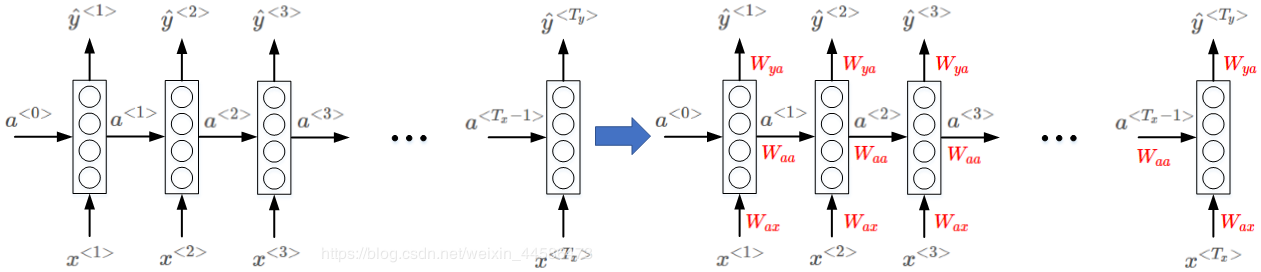 那么大家可能会产生疑问:这里看起来不是已经好多层了吗?怎么还是单层的?—— 其实,这就是 RNN 有别于 DNN, CNN 的一点了, RNN 的拓扑结构发生了很大的改变。我们需要明确一点:对于 RNN 而言,横向对齐的就视为同一层—— 这是因为:这一层所有的参数都是共享的!
既然谈到了参数,那么我们就有必要看看 RNN 是如何进行前向传播的:
RNN 需要有两个输入:
- 原本该时刻的单词输入 x < t > x^{
} x - 上一个时刻的激活值(或者说隐藏值) a < t − 1 > a^{
} a
我们这里的矩形框代表了类似于 DNN 里面的一个隐藏层,它执行的是下面的计算过程:
a < t > = t a n h ( W a a a < t − 1 > + W a x x < t > + b a ) y < t > = g ( W y a a < t > + b y ) a^{
那么,对于第一个时刻的输入,它确实有 x < 1 > x^{<1>} x<1>,但是此时并没有上一个时刻的激活值 a < 0 > a^{<0>} a<0>(因为现在就是第一个时刻)。此时我们可以给 a < 0 > a^{<0>} a<0> 赋值成 0 向量作为输入)
下面我们就以对句子: H a r r y P o t t e r a n d H e r m i o n e G r a n g e r i n v e n t e d a n e w s p e l l Harry\space\space Potter\space\space and\space\space Hermione\space\space Granger\space\space invented\space\space a\space\space new\space\space spell HarryPotterandHermioneGrangerinventedanewspell
进行名字识别为例,假设我们对每一个词用 10000x1 的词汇表进行独热编码,那么很容易想到,我们整个句子就是一个 10000 x 9 的矩阵: [ 0 0 ⋯ 1 0 0 0 0 ⋯ 0 0 0 ⋮ ⋮ ⋮ ⋮ ⋮ 1 0 ⋯ 0 0 0 ⋮ ⋮ ⋮ ⋮ ⋮ 0 1 ⋯ 0 0 0 ⋮ ⋮ ⋮ ⋮ ⋮ ] \begin{bmatrix} 0 & 0 & \cdots & 1 &0 & 0\\ 0 & 0 & \cdots & 0 & 0 & 0\\ \vdots & \vdots & & \vdots & \vdots & \vdots\\ 1 & 0 &\cdots &0 & 0 & 0\\ \vdots & \vdots & & \vdots & \vdots & \vdots\\ 0 & 1 &\cdots &0 & 0 &0\\ \vdots & \vdots & & \vdots & \vdots & \vdots\\ \end{bmatrix} ⎣⎢⎢⎢⎢⎢⎢⎢⎢⎢⎢⎢⎡00⋮1⋮0⋮00⋮0⋮1⋮⋯⋯⋯⋯10⋮0⋮0⋮00⋮0⋮0⋮00⋮0⋮0⋮⎦⎥⎥⎥⎥⎥⎥⎥⎥⎥⎥⎥⎤
假设我们的权值 W a x W_{ax} Wax 是一个维度为 100 x 10000 的矩阵。我们设 激活值的维度是 100 x 100, W a a W_{aa} Waa 的维度也是 100 x 100。根据式子: a < t > = t a n h ( W a a a < t − 1 > + W a x x < t > + b a ) a^{
如果我们把这两个权值合并为一个: W a W_a Wa,那么这个 W a W_a Wa 其实就是 W a a W_{aa} Waa 和 W a x W_{ax} Wax 的合并。合并方法就是水平合并: W a a = [ W a a ∣ W a x ] W_{aa} = [W_{aa} \quad|\quad W_{ax}] Waa=[Waa∣Wax]
如果我们把输入也合并成一个矩阵,那么应该是纵向合并: [ a < t − 1 > — — x < t > ] \begin{bmatrix} a^{
这样一来,我们 RNN 的激活值输出就可以简化地表示成: a < t > = W a X + b a a^{
看到这儿,可能大家又会有疑问了:RNN 的输出 y < t > y^{
我们现在就画出 RNN 一次前向传播完整的计算图: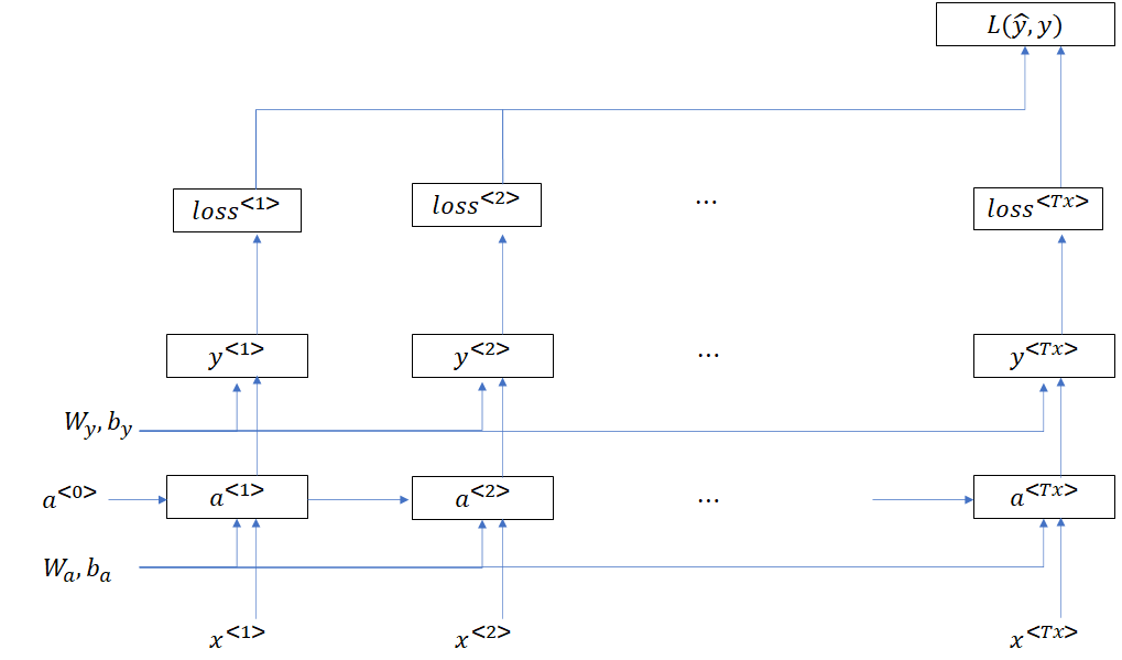
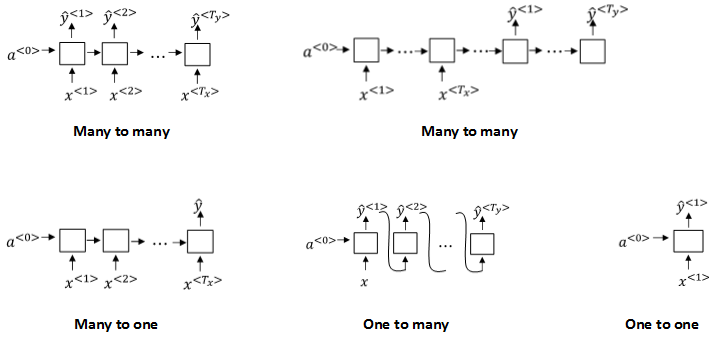
1.2.3 几种不同类型的 RNN
我们上面所讨论的是输入长度 T x T_x Tx 等于输出长度 T y T_y Ty 的情况,当然 也有 T x T_x Tx 不等于 T y T_y Ty 的情况——例如:多对多、多对一、一对多、一对一等等情况。我们可以根据需要再深入学习。
二、基于Pytorch的RNN实践部分
2.1 在Pytorch里面对 RNN 输入参数的认识
Pytorch 里面为我们封装好了 n n . R N N nn.RNN nn.RNN,每次向网络中输入batch个样本,每个时刻处理的是该时刻的 batch 个样本。我们首先来看看 Pytorch 里面 n n . R N N nn.RNN nn.RNN 的参数:
- i n p u t _ s i z e input\_size input_size :输入 x x x 的特征大小,比如说我们刚刚用一个 10000 x 1的词汇库去表示一个句子里面的其中一个词,所以,此时的 i n p u t _ s i z e input\_size input_size 就是 10000
- h i d d e n _ s i z e hidden\_size hidden_size: 可以理解为隐藏层神经元的数目
- n u m _ l a y e r s num\_layers num_layers: RNN 里面层的数量
- n o n l i n e a r i t y nonlinearity nonlinearity: 激活函数,默认为 t a n h tanh tanh,可以设置为 r e l u relu relu
- b i a s bias bias: 是否设置偏置,默认为 T r u e True True
- b a t c h _ f i r s t batch\_first batch_first: 默认为 f a l s e false false, 设置为 T r u e True True 之后,输入输出为 ( b a t c h _ s i z e , s e q _ l e n , i n p u t _ s i z e ) (batch\_size, seq\_len, input\_size) (batch_size,seq_len,input_size)
- d r o p o u t dropout dropout: 默认为0(当层数较多,神经元数目较多时, d r o p o u t dropout dropout 特别有用)
- b i d i r e c t i o n a l bidirectional bidirectional: 默认为 F a l s e False False , T r u e True True 则设置 RNN 为双向
上面的参数介绍里面提到了几个词: b a t c h _ s i z e , s e q _ l e n , i n p u t _ s i z e batch\_size, seq\_len, input\_size batch_size,seq_len,input_size 这该怎么理解呢?
比如说,我们还是以找寻句子里面的人名为例,但是这次的情况是:我一次给 RNN 输入3句话,每句话10个单词,每个单词用 10000维 的向量(10000 行的词汇表)表示。那么对应的 b a t c h _ s i z e batch\_size batch_size 就是 3; s e q _ l e n seq\_len seq_len 就是 10 ; i n p u t _ s i z e input\_size input_size 就是 10000.(值得注意的是: a e q _ l e n aeq\_len aeq_len 应该就是 RNN 的时间步)
说到这里,我们再举一个例子:
self.rnn = nn.RNN(input_size=INPUT_SIZE,hidden_size=32, # rnn hidden unitnum_layers=1, # number of rnn layerbatch_first=True, # input & output will has batch size as 1s dimension. e.g. (batch, time_step, input_size))
这样,我们就定义好了一个 RNN 层。
2.2 nn.RNN 里面的 forward 方法:
在对 RNN 进行前向传播时,注意这里调用的不是我们自己写的 f o r w a r d forward forward,而是 Pytorch里面 nn.RNN 的方法。具体格式如下:
rnn_out, h_state = self.rnn(x, h_state)
输入的第一参数 x x x ,它是一次性将所有时刻特征喂入的,而不需要每次喂入当前时刻的 x < t > x^{
输入的第二参数 h _ s t a t e h\_state h_state 是第一个时刻空间上所有层的记忆单元的Tensor,,只是还要考虑循环网络空间上的层数,所以这里输入的 s h a p e shape shape 是 [ n u m _ l a y e r , b a t c h _ s i z e , h i d d e n _ s i z e ] [num\_layer,batch\_size ,hidden\_size] [num_layer,batch_size,hidden_size]
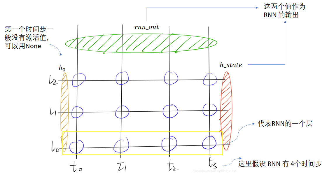
如上图所示,返回值有两个 r n n _ o u t rnn\_out rnn_out 和 h _ s t a t e h\_state h_state,其中,
r n n _ o u t rnn\_out rnn_out每一个时刻上空间上最后一层的输出(但是注意:这个输出不是我们所说的 y ^ \hat{y} y^,要产生 y ^ \hat{y} y^ 还需要我们再设计一个 n n . L i n e a r nn.Linear nn.Linear),所以它的shape是 [ b a t c h _ s i z e , s e q _ l e n , h i d d e n _ s i z e ] [batch\_size, seq\_len, hidden\_size] [batch_size,seq_len,hidden_size]
h _ s t a t e h\_state h_state 是最后一个时刻空间上所有层的记忆单元,它和 h 0 h_0 h0 的维度应该是一样的: [ n u m _ l a y e r , b a t c h _ s i z e , h i d d e n _ s i z e ] [num\_layer,batch\_size ,hidden\_size] [num_layer,batch_size,hidden_size]
Example:利用RNN进时间序列的预测
在本次的例子里面,我们的目的是用 s i n sin sin 函数预测 c o s cos cos 函数。主要还是为了熟悉 RNN 关于输入输出的一些细节。那么第一步就是导入必要的包啦:
import torchfrom torch import nnfrom torch.autograd import Variableimport numpy as npimport matplotlib.pyplot as plt
下面我们定义一些超参数:
# Hyper ParametersTIME_STEP = 10 # rnn time stepINPUT_SIZE = 1 # 说明一下:因为在每一个时间节上我们输入的数据就只是一个数据,并不像词那样用一个词汇表编码,所以这里input size就是1LR = 0.02 # learning rate
展示一下我们的数据:
# show datasteps = np.linspace(0, np.pi*2, 100, dtype=np.float32) # float32 for converting torch FloatTensorx_np = np.sin(steps)y_np = np.cos(steps)plt.plot(steps, y_np, 'r-', label='target (cos)')plt.plot(steps, x_np, 'b-', label='input (sin)')plt.legend(loc='best')plt.show()
下面是重点部分:我们开始构造我们的 RNN model:下面细节的解释都会在注释里面
class RNN(nn.Module):def __init__(self):super(RNN, self).__init__()self.rnn = nn.RNN(input_size=INPUT_SIZE,hidden_size=32, # rnn hidden unitnum_layers=1, # number of rnn layerbatch_first=True, # input & output will has batch size as 1s dimension. e.g. (batch, time_step, input_size))self.out = nn.Linear(32, 1) #说明:这里是 RNN 之外再加入的一个全连接层def forward(self, x, h_state):# x(输入)的维度就是(batch, time_step, input_size)# h_state (n_layers, batch, hidden_size)# r_out (batch, time_step, hidden_size)r_out, h_state = self.rnn(x, h_state) #注意:这里调用了nn.RNN的forward方法,输出两个,请看上文对它们的解释#print('第step次迭代, RNN所有时间结点上隐藏层的输出维度:', r_out.size()) #[batch, seq_len, hidden_len]outs = [] # save all predictions 这里我们需要定义一个空的列表,用于存放每一个时间节真正的输出(而不是r_out)for time_step in range(r_out.size(1)): # calculate output for each time step r_out.size(1)seq_len也即是时间节的长度outs.append(self.out(r_out[:, time_step, :])) #这里用[:, time_step,:]取出第time_step时刻的r_out作为nn.Linear的输入,用于计算该时刻真正的输出return torch.stack(outs, dim=1), h_state #最后我们需要把每一个时间节得到的output按照第二个维度拼起来
好的,在搞清楚 Pytorch 里面 RNN 的输入输出以及前向传播的计算过程之后,我们就要开始训练了:
rnn = RNN()optimizer = torch.optim.Adam(rnn.parameters(), lr=LR) # optimize all cnn parametersloss_func = nn.MSELoss()h_state = None # for initial hidden state 因为第1个时间节没有前一时刻的激活值,这里我们可以用None作为输入plt.figure(1, figsize=(12, 5))plt.ion() # continuously plotfor step in range(100): #训练100代start, end = step * np.pi, (step+1)*np.pi # time range# use sin predicts cossteps = np.linspace(start, end, TIME_STEP, dtype=np.float32, endpoint=False) # float32 for converting torch FloatTensorx_np = np.sin(steps)y_np = np.cos(steps)x = Variable(torch.from_numpy(x_np[np.newaxis, :, np.newaxis])) # shape (batch, time_step, input_size) 给 x_np加上第一个和第三个维度,都是1,因为这里默认batch = 1, input_size=1#print('x的维度:', x.shape) [1, 10, 1]y = Variable(torch.from_numpy(y_np[np.newaxis, :, np.newaxis]))#print('y的维度:', y.shape) [1, 10, 1]prediction, h_state = rnn(x, h_state)#Be careful!!!!#####h_state = Variable(h_state.data) # repack the hidden state, break the connection from last iteration#上面这一步我们需要把 RNN 第n次迭代生成的激活值作为下一代训练里面的 h0 输入,要重新打包成 Variableloss = loss_func(prediction, y) # calculate lossoptimizer.zero_grad() # clear gradients for this training steploss.backward() # backpropagation, compute gradientsoptimizer.step() # apply gradients#plottingplt.plot(steps, y_np.flatten(), 'r-')plt.plot(steps, prediction.data.numpy().flatten(), 'b-')plt.draw();plt.pause(0.05)plt.ioff()plt.show()
至此,我们应该对 RNN 的工作机理有了一个较为深入的了解。但是,在实际工程中,数据清洗与数据集的制作将会远远难于 RNN 本身的构造。这也需要我们有一个较深入的编程能力。虽然 Pytorch 等深度学习框架可以如此方便地自动计算梯度等等,但是数据集制作效果的好坏直接影响了我们 m o d e l model model 的表现。
然而,你以为故事到这儿就结束了吗?
如果我们现在的工作是让机器填词:假设我们给机器输入这样一段话: I a m C h i n e s e ⋯ ( 1000 w o r d s l a t e r ) ⋯ I c a n s p e a k f l u e n t _ _ _ _ _ I \space\space am\space\space Chinese \cdots (1000\space\space words\space\space later)\cdots I \space\space can \space\space speak \space\space fluent \space\space \_\_\_\_\_ IamChinese⋯(1000wordslater)⋯Icanspeakfluent_____
我们希望机器正确地填出最后一个词:当然希望是 C h i n e s e Chinese Chinese,然而假设中间这1000个词都和 C h i n e s e Chinese Chinese 没什么大关系,那么机器就需要记住句子一开始的 C h i n e s e Chinese Chinese。这无疑会给 RNN 反向传播带来极大的困难,可能会造成梯度消失。那么如何解决这个问题呢?—— 因此 L S T M LSTM LSTM 和它的变体 G R U GRU GRU 应运而生。
在之后的 B l o g Blog Blog 里面,我们会详细地学习 L S T M LSTM LSTM 的工作机理,以及如何在 P y t o r c h Pytorch Pytorch 里面实现 LSTM


还没有评论,来说两句吧...