matlab 图像分割 hough 霍夫变换-蒲公英云

matlab 图像分割 hough 霍夫变换

在此之前一般要边缘检测。

（1）hough变换原理

平面坐标系上直线转换到极坐标系上一个点，平面直角坐标系上点在极坐标系上为一条直线。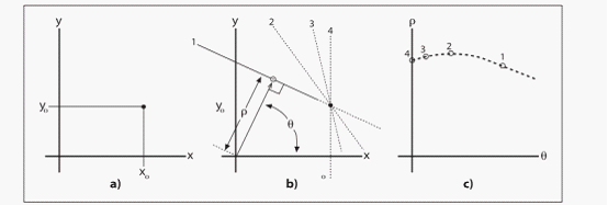
这里写图片描述

（2）有关函数介绍

1. [H,theta,rho] = hough(BW,p,v)

H是变换到的hough矩阵。
theta和rho对应于矩阵每一列和每一行的ρ和θ值组成的向量。
p与v成对使用。p如果使用thetaresolution则v是θ轴方向上的单位区间的长度，可取（0,90）之间，默认为1；p如果使用rhoresolution 则v是ρ轴方向上的单位区间长度，可取（0，norm（size(BW)）之间，默认为1。

2. peaks = houghpeaks(H,numpeak,p,v)

peaks是一个Q*2的矩阵，每行的两个元素分别是某一峰值的行列索引，Q为找到的峰值数目。
numpeak是寻找的峰值数目。
p和v成对使用。p如果使用threshold则v表示峰值的阈值，只有大于阈值的点才被认为可能是阈值，默认为0.5*max(H(:))。p如果是NHoodSize则表示每次检测出一个峰值后，v就指出该峰值周围需要清零的邻域信息，并以向量[M N] 形式输出。

3. lines = houghlines(BW,theta,rho,peaks,p,v)

lines是个结构数组，有point1（端点1），point2（端点2），theta,rho。
p和v成对使用。p如果使用fillgap则v表示同一幅图像中两条线的阈值，小于将会合并，默认20。p如果是minlength则v表示直线段最小长度阈值，默认40。
point1：两元素向量[r1, c1]，指定了线段起点的行列坐标。
point2：两元素向量[r2, c2]，指定了线段终点的行列坐标。
theta：与线相关的霍夫变换的以度计量的角度。
rho：与线相关的霍夫变换的ρ轴位置

（3）.完整代码：

RGB= imread('building.jpg');
I = rgb2gray(RGB);
BW = edge(I, 'canny');
[H, T, R]=hough(BW, 'RhoResolution',0.5,'ThetaResolution',0.5);
figure, imshow(imadjust(mat2gray(H)), 'XData', T, ...
'YData', R, 'InitialMagnification', 'fit');
xlabel('\theta'), ylabel('\rho');
axis on; axis normal; hold on;
colormap(hot);
peaks = houghpeaks(H, 15);
figure, imshow(BW);
hold on;
lines = houghlines(BW, T, R, peaks, 'FillGap',25, 'MinLength',15);
max_len = 0;
for k=1:length(lines)
xy = [lines(k).point1; lines(k).point2];
   plot(xy(:,1),xy(:,2),'LineWidth',3,'Color','b');
   plot(xy(1,1),xy(1,2),'x','LineWidth',3,'Color','yellow');
   plot(xy(2,1),xy(2,2),'x','LineWidth',3,'Color','red');
   len = norm(lines(k).point1 - lines(k).point2);
   if ( len > max_len)
      max_len = len;
      xy_long = xy;
   end
end

取出图中最长两条线：

I=imread('capture4.jpg');
BW=im2bw(I);
BW=edge(BW,'canny');
[H,T,R] = hough(BW);
imshow(H,[],'XData',T,'YData',R,...
'InitialMagnification','fit');
xlabel('\theta'), ylabel('\rho');
axis on, axis normal, hold on;
P = houghpeaks(H,10,'threshold',ceil(0.3*max(H(:))));
x = T(P(:,2)); y = R(P(:,1));
plot(x,y,'s','color','white');
lines = houghlines(BW,T,R,P,'FillGap',5,'MinLength',7);
figure,imshow(BW), hold on;
max_len = 0;
for k = 1:length(lines)
xy = [lines(k).point1; lines(k).point2]; %两点矩阵
plot(xy(:,1),xy(:,2),'LineWidth',2,'Color','green');
plot(xy(1,1),xy(1,2),'x','LineWidth',2,'Color','yellow');
plot(xy(2,1),xy(2,2),'x','LineWidth',2,'Color','red');
len = norm(lines(k).point1 - lines(k).point2); %两点距离
Len(k)=len
if ( len > max_len)  
max_len = len
xy_long = xy
end
end
plot(xy_long(:,1),xy_long(:,2),'LineWidth',2,'Color','blue');
[L1 Index1]=max(Len(:));
Len(Index1)=0;
[L2 Index2]=max(Len(:));
x1=[lines(Index1).point1(1) lines(Index1).point2(1)];
y1=[lines(Index1).point1(2) lines(Index1).point2(2)];
x2=[lines(Index2).point1(1) lines(Index2).point2(1)];
y2=[lines(Index2).point1(2) lines(Index2).point2(2)];
K1=(lines(Index1).point1(2)-lines(Index1).point2(2))/(lines(Index1).point1(1)-lines(Index1).point2(1));
K2=(lines(Index2).point1(2)-lines(Index2).point2(2))/(lines(Index2).point1(1)-lines(Index2).point2(1));
hold on
[m,n] = size(BW);
BW1=zeros(m,n);
b1=y1(1)-K1*x1(1);
b2=y2(1)-K2*x2(1);
for x=1:n
for y=1:m
if y==round(K1*x+b1)|y==round(K2*x+b2)
BW1(y,x)=1;
end
end
end
for x=1:n
for y=1:m
if ceil(K1*x+b1)==ceil(K2*x+b2)
y1=round(K1*x+b1)
BW1(1:y1-1,:)=0;
end
end
end
figure,imshow(BW1);